Well, this post suggests another method, using TempLS v2. TempLS was a program written last year, originally to provide alternative calculation of the main global temperature indices. It did that. It works on a different basis to most other such codes - instead of gridding anomalies, it fits a linear model to global temperatures by weighted least squares.
Version 2 extended this to fitting spatial variation parametrised by coefficients of basis functions, intended to be families of orthogonal functions like spherical harmonics. But the EOF's introduced by Eric Steig for the Antarctica analysis would do as well.
This post describes some preliminary results. There are some loose parameters which will need better definition. I have done almost no verification stats. The trends come out rather high. But the patterns are quite similar to the O10/S09 results. And their are some big plusses. One is simplicity - run times are a few seconds instead of the 40+ minutes I found with the RO10 method. And the simplicity means that one can experiment with more things - eg spatial weighting.
Review of TempLS
There is a description of the math in V1 here. There is a general overview of stage 1 of the project here. You can find a complete listing of old posts (by category) at the Moyhu index. Incidentally, I've had to move the document repository recently, so if you have trouble finding online materials, the new location is hereThe math description of V2 is here. In V1, global temperatures were represented by the model:
The data has a number of stations (s), with temperature readings (x) by year (y) and month (m). m varies 1:12. Then x can be represented by a local temperature L, with a value for each station and month (seasonal average), and a global temperature G depending on year alone.
xsmy ~ Lsm + Gy
This is fitted by area-weighted least squares. The weight function w is an estimate of the inverse of the local density ofstations. The local temp L includes the variations due to station location, including seasonal effects, leaving G to represent global influences.
In V2 this modelling was extended to allow G to include spatial variation. As a computing trade-off, it was no longer allowed to vary freely with year. Instead, the part of interest here (model 2) required that it vary linearly with year, so the trend could be estimated.
The model is:
xsmy ~ Lsm + J yPsk Hk
Here J is a linear progression in y; P is a set of values of k basis functions at s locations, and H are the set of coefficients to be found. I'm using a summation convention, so summed over k. In the present context P can be the values of the satellite EOF's.
Ground station results
The natural starting point would be to take x as the set of ground station temperatures. There were 109 ground stations in total, 44 manned and 65 AWS. However, 5 were omitted in O10 for various reasons, and are omitted here. I also excluded stations above latitude 60S, although I forgot to include this in the count shown in the trend plots. The total was then 99.TempLS would normally weight by area density, but since AFAICT S09 and O10 did not do that, I won't either at this stage. The normal scheme based on lat/lon cells gets a bit messy. So here is the standard TempLS output - the map of stations and the graph of numbers of stations in each year. All the analysis will be from 1957-2006. You can right-click to see the small pics in full size.
 Map of ground stations  Numbers reporting |  Trends |
On the right is a plot made using Ryan's plot routine for consistency (and because it's good). At the top are indicated some parameters (more explanation soon), and the trends for the Continent, and for the Peninsula, West Antarctica, and East Antarctica (see map). The main parameter of importance at this stage is that 6 EOFs were used.
Comparison
Here are some results described on Ryan's post, and from Eric at RealClimate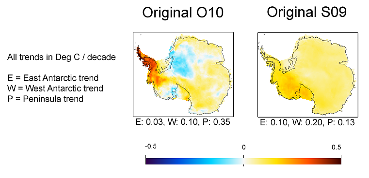 From Ryan's post  from Eric at RealClimate |
The TempLS pattern looks quite like O10's, but with larger trends in both directions. In the comparison, the continental trend was 0.06 for O10, and 0.12 for S09. So this value of 0.10 is in between. The Peninsula value of 0.56 is higher than both, as is the WA value, and EA is lower than both. But remember, the analysis so far was ground stations only
Use of AVHRR data
A key part of both S09 and O10 was infilling using both ground and AVHRR data. TempLS doesn't do infilling, but the natural equivalent is to add in artificial stations with AVHRR data. This was done with land/ocean indices - artificial stations created with SST data.We have 5509 AVHRR grid points, which gives more than enough coverage density. I reduced by a factor of 4 (leaving out alternate rows and cols in the rectangular grid of cells), making about 1392 in total. Theer will need to be relative weighting to prevent the ground stations being swamped, but for the moment I'll show the AVHRR stations only:
 Map of AVHRR "stations"  Numbers "reporting" |  Trends |
Mixing ground and AVHRR data
Now it's time to combine the data sets. There's no problem doing that - they are all in the same listing. The issue is relative weighting. If we want ground stations and AVHRR to have a roughly equal influence post 1980 (when both are available), then it would be appropriate to upweight the groundstations by a factor of about 15 (or maybe more, since ground stations have missing values, AVHRR generally not). So here is that case: Map of AVHRR "stations" |  Trends |
Again a pattern somewhat like that of O10, but with higher trends everywhere. The continent trend of 0.18 C/decade is very high.
Now it's time to explain the parameters shown on the trend plots. First is the number of ground stations, and then the number of AVHRR grids (though due to an error in the output program, this was underreported by 5). Then the weight factor, which is actually the number of extra times the ground stations are weighted (so if 15 is displayed, ground stations are upweighted by a total factor of 16). Then the number of AVHRR EOF's used as the basis functions. Finally, on the next line the trend values are reported.
Different weightings
OK, so we can try different weightings. I tried weightings of 8 and 40: Upweighting of ground stations =8 |  Upweighting of ground stations =40 |
The upweighting by 40 gives a pattern quite similar to O10. But again the Peninsula and WA trends are much higher.
Varying number of PCs
I've retained 6 EOFs above. The considerations seem to be similar to the S09 method. 4-6 looks like a good range, with noise problems increasing above 6. Here are the variations at weight factor 40: 4 EOFs |  5 EOFs | |
 6 EOFs |  7 EOFs | |
 8 EOFs |  9 EOFs |  10 EOFs |
Update. Here are plots of eigenvalues for the NxN matrix that has to be solved to get the coefficients (N=# PCs). I've shown N=5,7,10. The condition number is the ratio of largest to smallest. The max value of 53 for N=10 is getting large, but not disastrous.
 |
What still needs to be done?
A lot. I've done virtually no verification stats. Some sort of cross-validation is needed to get an optimal value of the weighting parameterhere the cost of departing from that is not prohibitive; the calc is currently a few seconds. But it would complicate the code.
(That isn't very accurate. The Santer/Quenouille correction affects the estimated error, which I haven't ventured yet. It wouldn't change the results quoted, although a fuller accounting for autocorelation would.)
And I could implement area-weighting. It's a bit complicated because of the differential weighting of the stations by type.
Update 27 May 2011
Kenneth Fritsch has been studying individual time sequences and breakpoints, as in the comments below. I'll link his graphics here:


Wow, I'm excited to see the cross-validation stats!
ReplyDeleteI was very impressed by TempLS - independent of benefits of the algorithm it just makes it much clearer what is going on.
I've only implemented Tamino's naive baseline algorithm myself, but have read about TempLS I proposed a modification of it which would give a poor-man's approximation to TempLS. Once you've got an initial estimate of global anomaly, you can go back and subtract this from all the station data. Then use all the data from the whole record to calculate new baselines. Iterate until stable.
Kevin C
Well done. It will be interesting to see if this method can lead to robust results once you do some cross-validation.
ReplyDeleteOne thing that seems increasingly obvious is that the original S09 paper significantly underestimate peninsular warming.
Zeke "One thing that seems increasingly obvious is that the original S09 paper significantly underestimate peninsular warming."
ReplyDeleteYep, it moved it onto the mainland...
Carrick,
ReplyDeleteWell, Nick's reconstruction has roughly equal trends to S09 for the mainland, though it should be taken with a strong grain of salt at the moment. The Peninsula differs the most in all alternative reconstructions.
Zeke, the most "no brainer" reconstruction of them all is Jeff Id's closest station reconstruction. Like O10, it concentrates most of the warming on the peninsula, and that is probably realistic, because that's what the actual station data says.
ReplyDeleteSo I wouldn't agree that "the Peninsula differs the most in all alternative reconstructions," at least without seeing a breakdown of trends + uncertainties for the various reconstructions.
Looks like a mix of the two, S09 underestimated the peninsular warming, O10 underestimated West Antarctica.
ReplyDeleteI agree that O10 probably underestimated WA warming. The question is by how much? My seat of the pants WAG is that by much less than the uncertainty quoted for their trend.
ReplyDelete(Based on my own experience with these sorts of regularizations, the bias is usually small compared to the rms noise in the data set.)
Nick,
ReplyDeleteGlad to see someone taking this on.
I would be very interested, since you've already got RO10s code running, to know what you get it you 'optimize' it -- using their methods -- for West Antarctica alone instead of all of Antarctica (which in my view is bound to mess things up in West Antarctica). I've not had the time to get into this.
I look forward to seeing what you come up with on this, and on your own TempLS methods.
Best
Eric Steig
Thanks, Eric. I'll do West Antarctica alone with TempLS - that's easy, although the data is sparser. Optimizing RO10 is more of a challenge, for while I can run the code, I still have a lot to learn about it.
ReplyDeleteI'm currently working on getting a good area weighting scheme, which may be relevant for WA.
Nick,
ReplyDeleteNice stuff. It's great to see the code being run.
Carrick points to a reconststruction by closest station above. That station simply combines anomalies with no offset trends are guaranteed to be slightly muted but whatever answers we get, they shouldn't differ a lot from that.
My favorite is the offset version in Fig 1 here http://noconsensus.wordpress.com/2009/08/31/area-weighted-antarctic-offset-reconstructions/
Anything much different than that is simply wrong in my opinion.
As to the comment thatO10 under or overestimates the trend in the west I think the arbitrary boundary of the PC's and the 'West' creates some difficulties. There is slight information shift in O10 as you would expect from the PCA dimensionality reduction. I believe the 'West' was within 0.02 C/Decade of the closest station offset reconstruction for the west. It has been 6 months though since I've checked, but I did check and it was close enough in all regions that I was unconcerned about overall accuracy of the publication.
Ryan has just placed a new post on line which addresses some other issues as well.
http://noconsensus.wordpress.com/2011/02/28/kgnd-cross-validation-by-ryan-odonnell/
Nick,
ReplyDeleteI had a post up but it disappeared. Links?
Carrick,
ReplyDeleteThe average percent variance retained for the RegEM ridge infilling is ~87%, and the retained variance following regularization for the AVHRR eigenvector inversion (using 126 eigenvectors) is ~88%. So if all of this bias translated into a reduction of trend in WA, a gross upper bound on the underestimation would be ~ 1 - sqrt(.88 * .87), or about 12.5% . . . which is, indeed, within the confidence intervals.
Jeff,
ReplyDeleteSorry about that - the blogspot spam filter is a nuisance. I check, but it's 7.30 am here. It doesn't seem to be links.
And Jeff, thanks for your comment. Ryan's post is going to keep me thinking today. I've been distracted by doing a tessellation for weighting - something you talked about a while ago.
ReplyDeleteAnd I see on looking that up that there is a new post at tAV for me to read.
Carrick,
ReplyDeleteMy recollection was that our main RegEM iridge infilled dataset retained an even higher proportion than Ryan states, of 98.4% of the maximum possible variance (being that which an unregularized ordinary least squares infilling would have retained). That allows for the fact that about half the data consists of actual rather than imputed values, and so retains 100% of the variance.
But maybe Ryan is referring to a different measure, or I have mis-remembered.
Ryan,
ReplyDeleteYes, there are posts on what TempLS is doing. Version 2, which is the extension to spatial models, is here. There is a more extensive explanation of the underlying LS model of V1 in this pdf, with an associated post here. There's an overview of development and applications here, now a little out of date. And there's the category index.
I agree with the point about the difference of trends between ground and AVHRR. That's why I varied the weighting ratio, which graduates from one extreme to the other. But even the ground stations give high values. It's always possible that I have just made an error with the data or some such. The verification process should shake that out, if so.
Nick,
ReplyDeleteWhat is difficult about the thing is the weighting by station per area rather than just bulk. The peninsula is heavily oversampled in comparison to the rest, this creates an artificial weighting in S09 and I believe in your images above which is the visible bleed through into the main continent of the peninsular trends that is not as prevalent in the closest station reconstructions.
If you reweighted the stations individually by area of influence (not sure how you would accomplish that - maybe distance to next closest station or something) my guess is that you might match O10 pretty closely.
Jeff,
ReplyDeleteYes, that's what I've been working on, via the Voronoi tesselation (post in next day or so, I hope). But it isn't easy to see what's right. What weight should Campbell Island, say, have? High if you count acres of Southern Ocean, nothing for its land area. I've been just leaving it out (so zero) claiming it's not Antarctic. But there's a similar problem for the peninsula tip.
I look forward to seeing the Voronoi Tessellation post.
ReplyDeleteA crude way to weight stations would be to simply draw a series of concentric circles around each station of say 50km radius, 100km, 200km, 400km, etc.
The weighting for each station is simply the fraction of land area in each circle, divided by the number of stations in the circle. The total weighting for the station is the sum of the weightings of all circles.
=======================
You would get a simlar sort of weighting by doing a series of passes with progressively coarser grids. Count the number of stations in each grid and that becomes the denominator for the weighting of those stations from that pass. Then multiply by the fraction of land area in the grid.
Both the concentric circle and coarsening grid methods depend upon the initial grid size / circle diameter chosen, and the multiplication factor for the step size. But working through a mental model of various combinations of station spacings, the algorithms seem to do what would be desired.
Of course, it will probably turn out that the Voronoi tessellation does a much better job, just as the Jeff's closest station method of reconstruction is simply a crude sanity check.
Nick,
ReplyDeleteYou may want to consider giving Campbell a zero weight. It's off the AVHRR grid (we did not use any stations as predictors that were not on the AVHRR grid).
Is there any mileage to looking at the cross correlations between time series for AVHRR grid points and using that to determine the area weighting?
ReplyDeletee.g. For each station, calculate the correlation between the nearest AVHRR timeseries and the timeseries for every other grid point in the map. (The same matrix used for the EOFs I guess). Then give that station a weight based on the number of grid points more strongly correlated to it than to any other station.
That's the kernel of an idea. I think you would also want a general cutoff, so if a map location is not correlated to any station better than some threshold then it doesn't get included in any weighting.
Some sort of fractional contribution would be better still.I wonder if there is a Bayesian approach to this?
Kevin C
Nick,
ReplyDeleteI have been unable to download TempLSv2.zip. The server at http://drop.io/erfitad doesn't seem to respond. Any chance of fixing this? I'm using Firefox 3.5.6
Thanks
NicL, drop.io is dead.
ReplyDeletehttp://blog.drop.io/2010/10/29/an-important-update-on-the-future-of-drop-io/
Killed by Facebook. Long live large corporations. (Or was that "drop dead").
NicL,
ReplyDeleteYes, I gave the new location in the "Review of TempLS section". You might as well download All-Files.zip (699 kb) - it's in there. I see I don't have it separately, but I'll fix that.
Kevin,
ReplyDeleteYes, something like that may be best. I've got the voronoi process producing areas, but there are still issues. Typically, if two stations are close, one has a big attached area, the other small, and so it is weighted out.
But there's another issue that affects all such attempts - it really needs to be done for each month, or at least updated frequently.
Kevin, fyi Roman did a post displaying spatial correlations from selected AVHRR grid points (processed with Comiso's cloud masking algorithm)here. Jeff also did a post
ReplyDeleteWhen will you have some confidence intervals to report with the trend numbers?
ReplyDeleteAlso it is interesting to see how the AVHRR data affect the warming trends.
I have already commented on verificatio/validation at TAV.
Kewnneth,
ReplyDeleteSoon, I hope. It's not as simple as an ordinary regression, because the error goes to the spatial solution, which is then averaged. But I'll do some simple stats very soon.
LL: Thanks for linking to the correlation pictures. They make interesting viewing. The East-West divide is startling!
ReplyDeleteKevin C
Nick, I do appreciate your stepwise approach which I think, although not stated, is your intent to show the effects of data inputs and usage. However, a result is never a result without the relevant uncertainties - even preliminary ones. I do appreciate the task required to calculate those confidence intervals.
ReplyDeleteI am curious at this point if your AVHRR only trends are in line with what we would have expected from the S(09) and O(10) had they used AVHRR only. O(10) used the AVHRR data for spatial reference and not temporal (as in trends). You show a very warmed Antarctica with AVHRR data and trends from 1957-2006. But we know that no AVHRR measurements existed for nearly the entire 1st half of that time period. Your calculation therefore requires you to "fit" the AVHRR data from the latter period to the ground data of the earlier period. How do you calibrate the AVHRR data to the ground data?
Do AVHRR temporal elements (trends) enter into your calculated ground trends? That was not clear to me.
Nick Stokes: "I've got the voronoi process producing areas, but there are still issues. Typically, if two stations are close, one has a big attached area, the other small, and so it is weighted out."
ReplyDeleteThat's also a problem with using a "closest station" approach of assigning area. The only concept I've found that does what I want is do counts of stations in successively larger areas and combine those multiple weightings.
You're welcome Kevin. Of course the "startling" east / west divide correlation differences come when correlating grid points from the S09 reconstructions like this, this, and this. The corresponding plot using actual AVHRR data is here.
ReplyDeleteNick Stokes, I am posting to determine if your blog is still active as I have not seen any communication for a few days.
ReplyDeleteI had asked some questions of your methods at Post#30. Is there any chance that you might answer those questions? I am guessing here that your results depend heavily on the trends from the AVHRR data and I would like to understand better the differences between your methods and S(09) and O(10) with regards to the AVHRR data.
Also can you provide a quick status on determining CIs for your trends and validation/verification statistics for your method?
Kenneth,
ReplyDeleteYes, it's still active, and I apologize for the delayed response. I'm about to post the Voronoi area-weighted results for Antarctica, and you'll be pleased to know they do produce some lower trends.
I'd been hoping to have confidence intervals before now. It's complicated by the method of calculation, in which the spatial approximations are computed first, and then the space-averaged trends. So there's a spatially dependent uncertainty as an intermediate. My guess at this stage is that the CI's will be similar to O10 and S09.
The difference between AVHRR and ground is crucial, and as Ryan has observed, deciding which you have faith in has a big influence on the result you reach. This is basically not a statistical question, as there is no third validation source. If you emphasise ground tests in validation, you'll get a ground-dominated result.
My approach was simple mixing. As the diagrams indicated, the AVHRR cells (or a subset) were entered as if they were ground observations in the LS fitting, but with a relative weighting factor, which I can vary. That loose parameter is one reason why I don't think too much notice should be taken of the trend magnitudes at this stage.
There is no separate calibration of the AVHRR cells required - the LS method takes care of that. As with ground stations of various altitudes etc, calibration goes into the L local variation parts of the model, which are distinguished from the regional effects by the hypothesised lack of year tgo year variability.
O10 and S09 used a more complicated infilling process to blend the effect of AVHRR and ground stations. At this stage I don't have a good theoretical view as to how the effect of this difference would appear in the results.
I've given priority at this stage to resolving the spatial weighting issue because I think it may have a significant effect on the result.
Thanks for the reply, Nick. It is good to see other methods applied to the Antarctica temperature data. From my excerpt from your post below I am wondering whether you are convinced that O(10) showed good evidence that the AVHRR was not reliable or stable in the temporal mode as the satellite sensors analysis indicated they were not stable over time. That drift I have assumed would not preclude stability over space at a given time. Is it really a matter of faith which measurements you use for extracting temporal information or can a reasonable analysis guide the way?
ReplyDeleteAnd by the way if your method is not optimum for extracting temperature trends I would not accept a result from you that showed lower trends than O(10). Maybe you were judging/anticipating my reactions based on Eric Steig's insistence on a warming WA.
"The difference between AVHRR and ground is crucial, and as Ryan has observed, deciding which you have faith in has a big influence on the result you reach. This is basically not a statistical question, as there is no third validation source. If you emphasise ground tests in validation, you'll get a ground-dominated result."
Nick, a couple of further questions and that is do you really think AVHRR data, a skin temperature, and ground stations, an air temperature, can be used interchangeably and without calibration one to the other? Have you looked at the relationship of AVHRR to ground stations? Or does you method somehow take into account the relationship?
ReplyDeleteKenneth, that's the fumction of the local temp L in the linear model. It fits that by LS to each source, whether its a sea level ground station, a mountaintop, or a satellite. The trend is the next effect. In my next post I'll be showing residuals which should make that clearer.
ReplyDeleteRomanM talked about this in a series of posts like this. The LS provides an offset, which is what calibration would do.
Kenneth,
ReplyDeleteJust following up on your other question about time stability of AVHRR. I haven't taken this any further than O10, who I think left it that they would use the data, but felt that it needs watching. As I said above, I think the relative merits of AVHRR and ground are debatable, but can't be resolved by statistics alone.
Nick, I need to look in more detail how your method applies to the AVHRR and ground data in the Antarctica - for my own understanding. My gut feeling is that an algorithm that might correctly apply to extracting global and regional temperature trends from more or less homogenous temperature readings and readings homogonized over time could have problems without major adjustments doing it with the AVHRR and ground data.
ReplyDeleteI did some background reading on your methods as applied to global and regional temperatures, but I was not sure how well they performed. I recall seeing some comparisons at Zeke's blog where all the methods compared reasonably well, including your method. Also I assume that when you made your global and regional calculations that you used adjusted temperature data from for example, GHCN.
Kenneth,
ReplyDeleteThe method is really just linear regression. It doesn't modify the data, but fits to it as read from file. On GHCN, I can use the adjusted file, or the raw file - I always use the raw file. When mixing data, I just handle them as separate stations - earlier with SST, now with AVHRR. Because the linear model has a term with monthly offsets, fitting that term handles the issues of possible offsets between the records.
As to analyses that I've done with results that can be compared to - yes, the posts of Zeke were the most comprehensive and quantitative. For example, land only, land-ocean. I don't think any of these analyses established that any one method was better - just that they all got equivalent results within the error range, incl TempLS. On the spatial methods of V2, used here, it's harder to get numerical measures, and I haven't found blogger results to compare with. But there are global comparisons (more here, and regional.
"The method is really just linear regression. It doesn't modify the data, but fits to it as read from file. On GHCN, I can use the adjusted file, or the raw file - I always use the raw file. When mixing data, I just handle them as separate stations - earlier with SST, now with AVHRR. Because the linear model has a term with monthly offsets, fitting that term handles the issues of possible offsets between the records."
ReplyDeleteAlthough I am woefully deficient in linear algebra, I think I follow your explanations there and I have no reasons to doubt your correctly applying the algebra. It is the assumptions that I think you are making that I have to understand better.
In your reply comment above you say that you use the raw file which to me, in the case of GHCN would imply that you use data that is not adjusted for TOB, UHI and other homogeneity factors. I think this would produce a big difference between raw and adjusted data for GHCN in the US. Are you saying that your method is then compared to adjusted data and compares favorably? If it does then your method would appear to be somehow adjusting for the homogeneity factors directly.
You also show trends from 1957-2006 using AVHRR data that predate the existence of AVHRR data. Your model equation has a local partition and a global one for the station result. You state that the AVHRR EOFs are used in the global part and that the ground stations are consider x. Obviously the number of ground stations varies over time but some do extend back over time to 1957. Without the AVHRR data before 1980, or so, the global partition disappears unless that part remains attached to AVHRR EOFs derived from the 1980-2006 data. I guess that would be the only logical explanation. I can certainly see the spatial relationship extending to the pre-AVHRR existence but I cannot see how the temporal part can and if it cannot then how would you link the before and after data?
Kenneth,
ReplyDeleteGHCN publishes its v2.mean etc database which now comes directly and without adjustment from the met data submitted on CLIMAT forms from met orgs around the world. They also publish an adjusted database, described by Peterson and others. AFAIK, no major organization uses that adjusted data. I didn't in anything on the blog. Zeke looked at the effect of USHCN adjustments, and comparison with GISS where they used adjusted data. There wasn't much effect. I found similar things in experiments that I didn't blog on.
On AVHRR, Steig's idea was that, while we only have recent data, it's reasonable to assume that the spatial pattern was similar in the past. That is reflected in the use of the eigenvectors as basis functions for both recent and pre-1980 data. Having chosen the basis functions, the fitting still proceeds for both AVHRR and ground data (in combination). Before 1980, the fit is only influenced by ground data - after that by both (how much of each is determined by the weight factor that I discussed).
Nick, there are adjustments to v2 version of GHCN with the pairwise homogeneity algorithm which includes identifying statistically significant break points between stations within reasonable correlation distances. I take it you use version 2 data. And Zeke compares that result to version 2.
ReplyDeleteftp://ftp.ncdc.noaa.gov/pub/data/ghcn/v2/source/inhomog/README.homogeneity
"Current homogenization is done with the Pairwise Homogeneity Algorithm
used in the US Historical Climate Network"
Nick, I was curious whether you have attempted to test the limits of your method by removing data from a reasonably complete data set and seeing what happens to the calculated trend from that calculated for the more complete data set. Would you expect that deterioration to be different depending on the size of the area covered?
Kenneth,
ReplyDeleteI think that "current homogenization" line is referring to GHCN v3, as that was the major change made going from v2 to v3. While there was an GHCN v2 adjusted file (v2.mean_adj), I believe they used the Peterson and Easterling programs rather than the PHA.
As Nick mentions, few folks use the v2.mean_adj file, and instead use the unadjusted v2.mean file. This may start to change now that v3 is out.
I should caveat my statement that "few folks use the v2.mean_adj file" to add that GISS (and maybe HadCRUT?) does use adjusted USHCN data for the CONUS. I don't recall if they just ignore GHCN data for the U.S., or if it completely overlaps with the USHCN network.
ReplyDelete"The following programs (pe.f, ep.f, adj.mon.f) were written by
ReplyDeleteDr. Thomas Peterson and Dr. David Easterling and were used to adjust
Global Historical Climatology Network (GHCN) v2 data. The pe.f program
used a proprietary sort routine and thus it has not been redistributed
with the source code file, so users will need to introduce their
own sort routine.
Current homogenization is done with the Pairwise Homogeneity Algorithm
used in the US Historical Climate Network. Information and code may be
found at:
ftp://ftp.ncdc.noaa.gov/pub/data/ushcn/v2/monthly/software/"
The complete excerpt indicates that it is referring to GHCN v2. Certainly we know that USHCN v2 was adjusted with pairwise breakpoint analysis. Also that if you look at 1920 forward that the USHCN v1 and v2 versions give statistically significant differences in trends - not by much but significantly different. I can also select periods where the differences are not significant.
Kenneth,
ReplyDeleteI'm not sure what you are getting at with the Peterson quote. The GHCN v2 data includes files that have been adjusted with those algorithms - they are indicated with a _adj suffix. The others, which we use, haven't.
Sorry about the slow answer on your other qn - I've been trying to work out what is appropriate. The main test of that kind, I guess, was the 60 stations exercise (which I have been redoing with Voronoi - post soon). But there has been a lot of subsetting. Another example would be the GSOD/GHCN comparisons - not exactly subsets, but 2 datasets covering the same region.
"The others, which we use, haven't."
ReplyDeleteI am attempting to learn what is claimed for your algorithm or anyone else's that uses the raw data. Can I assume that if you were to use the raw GHCN data for the US, as in USHCN v2, you would compare your resulting adjusted data with the adjusted data for USHCN. The USHCN v2 adjusted data is adjusted separately for TOB and then makes the pair wise homogeneity adjustments.
In these comparisons is the claim that your algorithm adjusts for TOB and pairwise homegeneity that USHCN makes on the raw data given you obtain a good agreement with the adjusted data.
I thought that perhaps you used the adjusted GHCN or USHCN with your algorithm with the idea of making improvements in how the missing spatial and/or temporal data was used. If you use raw data then I assume that your algorithm covers all the adjustments made by GHCN/USHCN and the final comparison is adjusted to adjusted.
Kenneth,
ReplyDeleteThe algorithm I'm describing doesn't adjust anything. It simply takes a set of supplied temperatures and fits a linear model. It's a fancy linear regression. Regression doesn't adjust anything - it calculates a trend.
And all I'm saying is that I use the published unadjusted datasets. It's possible to compare the calculated trends of adjusted and unadjusted data, for example. Zeke did some of that.
The fitting doesn't attempt to compensate for inhomogeneities. My own feeling about that is that for global calcs a large amount of data is being averaged, and inhomogeneities will tend to cancel. Adjusting introduces lots of false positives, but they tend to cancel too. The argument for adjusting is basically that the false positives are more likely to be unbiased than the apparent inhomogeneities corrected. I think that is likely, but probably not worth the hassle.
Nick, I think I know what your algorithm does and my choice of adjustment was probably poor. Specifically what I am attempting to get at is that I know that over a reasonably long time period that the adjustments of the adjusted USHCN temperature series account for a large part of the trend in the ajusted series.
ReplyDeleteIf I compare the adjusted and raw USHCN series for long term trends I will see a difference with the adjusted trend being the larger. Have you applied your algorithm to the raw data from USHCN and if so how well did it compare with the trends from the USHCN raw and adjusted data series?
The second graph in the linked article below shows the difference in trends between the USHCN adjusted and unadjusted temperature data. I also assume that when you and Zeke refer to raw data you are referring to unadjusted data. It is that difference that I am curious about as to what your algorithm working on the unadjusted data will give as a result - in comparison.
ReplyDeletehttp://cdiac.ornl.gov/epubs/ndp/ushcn/ndp019.html
Kenneth Fritsch,
ReplyDeleteYour link refers to USHCN v1, rather than v2, so its slightly outdated. For version 2, this is the relevant paper: ftp://ftp.ncdc.noaa.gov/pub/data/ushcn/v2/monthly/menne-etal2009.pdf
It appears I am not getting my answer on the use of the Stokes algorithm. I'll ask if the use of the algorithm for a given set of data is simply that it yields similar results without the need for gridding the data and deals with missing data more efficiently?
ReplyDeleteZeke, I am well aware of the v1 and v2 versions of USHCN and also that v1 and v2 give much closer trends than v1 compared to raw (unadjusted) data. Therefore, the differences between trends from raw (unadjusted) USHCN and v2 data will be large, also, and I think perhaps slightly larger for v2.
Kenneth,
ReplyDeleteSorry I missed that - no I haven't applied the algorithm to USHCN specifically. I have done a US analysis but with GHCN data.
I don't think TempLS would add anything there. NOAA has published on the effects of the various adjustments (raw vs adjusted, in stages). He says the effects are quite large, and it seems that it is that high level that critics focus on, rather than doubting NOAA's analysis.
Nick, can you update the status on applying your algorithm to the Antarctica temperatures?
ReplyDeleteKenneth,
ReplyDeleteWell, there are two new posts - area weighted trends, and non-EOF trends. I think area-weighting is a big improvement. But they all seem to give fairly similar results.
But mainly I've been concentrating on releasing the new version. People can now run the code themselves.
While contemplating Nick Stokes' algorithm for in-filling Antarctic temperature data from ground station and AVHRR satellite grids, I decided to download all the data series from O(10) including the RLS and EW reconstructions used in O(10), the S(09) reconstruction featured in S(09), and referred to hereafter as S09, and the raw (after cloud masking) AVHRR data. Also included were the ground station data from the manned and AWS stations.
ReplyDeleteI was primarily interested in the 1982-2006 period as I wanted to make comparisons with the AVHRR data that became available during that period. The downloaded data was put into monthly anomaly form based on the 1982-2006 time period. In my analysis I used 50 of the ground station data that were most complete for that period and further were within the area covered by the AVHRR grids.
The RLS method in O(10) uses only the spatial component of the AVHRR data for in-filling the missing ground station areas, while the EW method in O910) uses both the temporal and spatial relationships between ground stations and AVHRR data.
The S09 method uses RegEM and combines ground and AVHRR data. A major part of the S09 methodology involves the retention of just 3 AVHRR PCs.
In my initial analysis of these data sets I have included correlations and trends of these data using latitude, longitude and altitude as explanatory variables. I must admit that I was surprised at how influential these variables turned out to be. In think that perhaps a better regression would have used a reference point and distances from it, but in the analysis presented below I simply used latitude, longitude and altitude as taken from the downloads from O(10).
This thread has discussed the effects of Chladni patterns on a PCA that retains just a few PCs and I thought perhaps the differences I saw between the O910) and S09 methods with regards to latitude and longitude and possibly altitude might be related to the effects of Chladni patterns.
RLS does not use AVHRR PCs, while the EW method use 150 AVHRR PCs as compared to S09 which uses only 3 AVHRR PCs. In the linked first two tables below it can be seen that, when regressing trends or correlations versus latitude, longitude and altitude, overall S09 is more influenced by these variables than are the RLS and EW reconstructions. The questions that arise in my mind are if you see a change in influence of these variables from the raw data to that data reduced to a few PCs is that change one that you might observe because the PCs are eliminating sufficient noise or are the changes a matter of an influence of geometry that might be considered spurious?
While the ground station data is limited, it is interesting to look at the correlations and trends of the reconstructions and AVHRR data (nearest grid to station coordinates) versus the ground stations (linked below in the 4 tables in the second link below). We can see that the RLS reconstruction gives the best correlation at 0.96 and EW next at 0.87, the S09 lags far behind at 0.49 and the AVHRR data is in the middle at 0.71. The same order exists for the regressing trends of AVHRR versus the RLS, EW and S09.
In the linked tables we can see that, although the data are small, the ground station and corresponding AVHRR data when regressed as trends and correlations show little or no influence from the latitude, longitude and altitude. The influence of these explanatory variables is seen to a greater extent in the O(10) and S09 reconstructions with by far the greatest influence being seen with the S09. The ground station data generally confirms what is seen in the analysis that uses all the AVHRR grid point data for all the reconstructions.
http://img695.imageshack.us/img695/9256/rlsews09avhrraltlatlon.png
http://img10.imageshack.us/img10/3707/groundstatrlsews09avhrr.png
Kenneth,
ReplyDeleteThat is very thorough analysis. One thing I had been wondering is the difference between spatially fitting temperature and then computing the trend, vs calculating the trend locally, and then spatially fitting that. You're doing something like the latter.
Would you be interested in gathering this together as a head post here? Tables and diagrams could be properly displayed. If you wanted to make a HTML file, I could put it up, or I could probably give you authority to work on the site editor directly?
Thanks for the offer, Nick, but I would rather see if there is any interest in what I did here based on what I have currently presented or anyone who might show any errors in my analysis and/or thinking. I would be happy to show more of the details of what I did in separate posts if anyone is interested.
ReplyDeleteI think I understand your question in the post above and I can show you where the differences in calculations methods for the regional trends will have insignificant differences on the final results.
My analysis was being directed towards attempting to determine the differences in trends by using the non calibrated AVHRR data versus the ground stations data combined with the spatial relationship of the AVHRR data to the ground stations. When I saw the effect of latitude, longitude and altitude on the regressions I was doing, I started to think about Chladni patterns and in effect temporally got off the subject.
I continue to think that for your analyses you need to determine whether the AVHRR data or the ground station data better represent the temperature (anomalies) in the Antarctica. I think weighting the two sources could be misleading and also presents the dilemma that if the AVHRR data is correct than you can no longer use the ground station data from pre-1982 and you are left with only the 1982-2006 (or later to present if you use data beyond what S(09) and O(10) used). By truncating the analysis you also run into the problems of the reduced data set not producing statistically significant trends.
It has always been my contention that the S(09) authors were primarily interested in showing statistically significant trends for the regions of the Antarctica and the continent as a whole - if they existed. In order to do that they had to depend on the temporal part of the ground stations. Now if one can show that the ground stations and AVHRR temporal results are different, one must then choose the ground station as the appropriate source in both pre and post AVHRR measurements to get the 1957-2006 trends (AVHRR could be calibrated with the ground station data) or choose AVHRR as the appropriate source and limit the analysis and trend calculations to the 1982-2006 period.
The RLS reconstruction of O(10) seems to fit better what S(09) intended as it uses none of the temporal AVHRR data. The EW reconstruction from O(10) does use temporal AVHRR data but with different methodologies and very different results than S(09) but similar to RLS. The EW method calibrates AVHRR data to ground station data, but as I recall, the authors do not claim this accounts for any significant differences in results with S09. O(10) uses over 100 AVHRR PCs for EW whereas S(09) uses 3. O(10) also claims to use optimal determination of regularization and proper determination of spatial structure during infilling.
I was hoping that a breakpoint analysis of the difference series between AVHRR and RLS for all 5509 grid points would reveal something, but that is a very slow process of which I have only covered 1/5 by running my computer all night. Today I want to look at difference series for entire regions of the Antarctica.
Kenneth,
ReplyDelete"O(10) uses over 100 AVHRR PCs for EW whereas S(09) uses 3."
There's more to that story. I found that if you go over about 10 or so PCs, the results get ragged. Too much noise. So 100 PCs on its own is a bad idea.
I understand O10 used Tikhonov regularisation for EW. This reduces noise by reducing effective DOF. Higher PC's contribution is damped. Their kgnd is equivalent in effect to, I believe, about retained 7 PC's.
Based on your comment above, Nick, the point of using the raw cloud masked AVHRR data comes to the fore. If the AVHRR data are an appropriate proxy for Antarctica temperatures, then we have temperature measurements or a proxy for such with the AVHRR data for all of Antarctica. S09 uses 3 AVHRR PCs and your algorithm uses 6 PCs. The more PCs you use the closer you come to getting back the original data - and with all its noise. I have been using the raw cloud masked data in my analyses and particularly in a comparison with RLS for the period 1982-2006. Would these analyses and comparison be somehow invalidated because the original AVHRR data is too "noisy"?
ReplyDeleteWhat you are referring to above is that the noise problem from the use of higher numbers of EOFs of the AVHRR data comes from your algorithm. I understand that you follow that by saying that O(10) mitigates the noise of the use of many EOFs by the use of Tikhonov regularization and choice of retained kgnd parameters.
Your method, that I used, allowed only the use of 15 EOFs and I found that the changes from using 3 or 15 were not that much different for the entire continent when using a 100% weighting for AVHRR. The changes were more pronounced on increasing the number of EOFs used when using 100% weightings for ground stations and in the progression from the Antarctica continent, East Antarctica, Peninsula to West Antarctica.
I wanted to show in a post today the breakpoints for the difference series of AVHRR-RLS during the period 1982-2006 for the continent and the 3 major regions of the Antarctica.
Further to my post above: are you saying that if the EW reconstruction were performed using 7 AVHRR EOFs with some other regularization algorithm that the results would have been essentially the same?
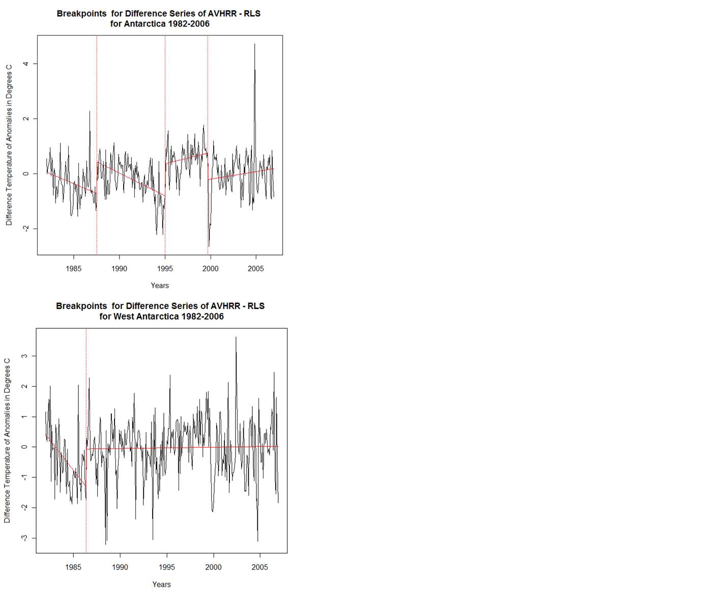
ReplyDeleteBelow are linked four graphs showing the breakpoints for the Antarctica, East Antarctica, West Antarctica and the Peninsula for the difference series AVHRR-RLS for the period 1982-2006. I have not attempted to associate these breakpoints with any events, but the fact that you can find statistically significant linear segments in a difference between temperature series is an indication that one or both series were not accurately portraying temperature over the period of interest. This procedure is essentially the same as that used by USHCN to find non homogeneities in the US temperature records.
ReplyDeleteA linear regression for the entire time period for the areas above and for AVHRR-RLS shows a positive and statistically significant trend for the Antarctica, East Antarctica and West Antarctica while the Peninsula trend was not significant.
http://img864.imageshack.us/img864/8076/antarcticavrlsbps2h.png
http://img809.imageshack.us/img809/8358/antarcticaavrlsbvps1.png
I should be concise above in that the USHCN method looks at difference series between nearby stations whereas I am looking at entire regions. Finding breakpoints under the conditions I used should be more meaningful then that under which USHCN declares homogeneity differences as under the conditions of my calculation, with a large number of stations (grids), random errors can cancel out.
ReplyDeleteThanks, Kenneth,
ReplyDeleteApparently Blogger doesn't allow images incomments, so I've appended them to the post above.
I have completed some more breakpoint/breakdate analysis of the Antarctic difference series and report the results below in a summary of all the difference series. All series are for the 1982-2006 period.
ReplyDeleteS09-RLS:
Antarctica: Aug 1987, Jan 1995 and Sep 1999
East Antarctica: Aug 1987 and Jan 1995
West Antarctica: May 1986 and Aug 1998
Peninsula: Nov 1985
AVHRR-RLS:
Antarctica: Aug 1987, Jan 1995 and Sep 1999
East Antarctica: Aug 1987 and Jan 1995
West Antarctica: May 1986
Peninsula: Sep 1999
RLS-EW:
Antarctica: None
East Antarctica: None
West Antarctica: None
Peninsula: None
AVHRR-S09:
Antarctica: Oct 1993
East Antarctica: None
West Antarctica: None
Peninsula: None
All the regional 1982-2006 period linear trends for the AVHRR-RLS difference series were significant except for the Peninsula, while for AVHRR-S09 and RLS-EW none of these trends were significant. For S09-RLS difference series the Antarctica continent and East Antarctica had significant trends but not West Antarctica and the Peninsula.
For the period 1982-2006 it appears that the differences between S09 and the two O(10) reconstructions are very much influenced by the AVHRR data and by differences that produce statistically significant linear segmentations (breakpoints). If RLS is a good proxy for the ground stations, one might deduce that differences between reconstructions of S09 and O(10) are differences heavily influenced by differences between satellite and ground measurements. I can do some breakpoint analysis of the more complete ground station series as difference series with the corresponding AVHRR, S09 and RLS grid data for the 1982-2006 period.
In my spare time I have looked at regional ground station series break points for comparing with the those for RLS, EW, S09 and AVHRR in an attempt to determine whether the ground stations are similar in breakpoints with RLS and EW or S09 and AVHRR. Remember that RLS grids corresponding to ground stations had a very high correlation, followed by EW and then AVHRR and finally S09.
ReplyDeleteFor the period 1982-2006 I took the averaged monthly data (300 months) for the 13 ground stations, with near complete data, and RLS, EW, S09 and AVHRR series. I calculated breakpoints for the Antarctica continent and the three major regions. The results are as follows:
Ground Stations:
Antarctica: None
East Antarctica: None
West Antarctica: None
Peninsula: April 1986, Feb 1990
RLS:
Antarctica: None
East Antarctica: None
West Antarctica: None
Peninsula: April 1986, Jan 1990
EW:
Antarctica: None
East Antarctica: None
West Antarctica: None
Peninsula: April 1986, Jan 1990
AVHRR:
Antarctica: Oct 1990, Jan 1995
East Antarctica: Sept 1990, Jan 1995
West Antarctica: None
Peninsula: None
S09:
Antarctica: Oct 1990, Jan 1995
East Antarctica: Sept 1990, Jan 1995
West Antarctica: None
Peninsula: None
From these results one can further see that RLS and EW are closely related with regards to breakpoints and S09 and AVHRR are closely related but not related to RLS and EW. RLS and EW are closely related in breakpoints to the grounds stations.
When I looked at individual difference series between ground stations and their corresponding grids for RLS, EW, S09 and AVHRR, I found that rather random breakdates occurred in approximately 40% of the difference series. The occurrence of breakpoints of the difference series had no apparent effect on the correlation of the two series used for the difference. I found that observation almost going against conventional wisdom and needing more thought and analysis about what it might be telling us.
When I have time I want to now look at comparing the various sources of temperatures for the Antarctic regions such as the UAH TLT data and the Steig data from ice cores in hopes of further elucidating which data series: AVHRR or ground stations better reflects the true Antarctic temperatures.
I have been attempting to determine whether a change in the AVHRR data can be related to instrument changes. The changes are linked here:
http://www.neodc.rl.ac.uk/?option=displaypage&Itemid=122&op=page&SubMenu=-1
A change does correspond with the Jan 1995 breakpoint but none to the Sep/Oct 1990 breakpoint.
I found some time to load the UAH monthly gridded temperature data from 1982-2006 into R and compare it to the monthly RLS, EW, S09 and AVHRR series over the same time period. The UAH grids can encompass from 1 to 12 of the 5509 AVHRR grids. We also know that the UAH satellite measurements are claimed not to replicate well the polar temperatures at the highest latitudes, but since these is a comparison of all the series in question to UAH I used all the available UAH data as published.
ReplyDeleteThe UAH to other four series comparisons were made (a) using the mean and standard deviation of the correlations performed on a grid to grid(s) basis and (b) using the monthly means over the entire 1982-2006 period for all the series and differencing the UAH series with4each of the other four series and (c) determining the trends for these difference series as well as a breakpoint calculation for the difference series.
The results are summarized below:
Grid to Grid correlations:
UAH to RLS:
Average correlation =0.675; Standard deviation of correlations=0.102
UAH to EW:
Average correlation =0.673; Standard deviation of correlations=0.107
UAH to S09:
Average correlation =0.638; Standard deviation of correlations=0.101
UAH to AVHRR:
Average correlation =0.607; Standard deviation of correlations=0.113
Trends of Difference Series are in degrees C per decade and correction to SE for trend slope was calculated using the Nychka method for AR1:
UAH-RLS:
Trend Slope=-0.114; AR1=0.232; Adj. SE Trend Slope=0.0636; Significant slope at 5%: No
UAH-EW:
Trend Slope=-0.058; AR1=0.323 ; Adj. SE Trend Slope=0.0613; Significant slope at 5%: No
UAH-S09:
Trend Slope=-0.294; AR1=0.476 ; Adj. SE Trend Slope=0.0952; Significant slope at 5%: Yes
UAH-AVHRR:
Trend Slope=0.295; AR1=0.468 ; Adj. SE Trend Slope=0.0952; Significant slope at 5%: Yes
Breakpoints of Difference Series:
UAH-RLS:
Breakpoints: None
UAH-EW:
Breakpoints: July 1987
UAH-S09:
Breakpoints: Dec 1988, Jan 1995, Sep 1999
UAH-AVHRR:
Breakpoints: Dec 1988, Jan 1995, Sep 1999
The results above point to, once again, the RLS and EW series pair being alike in these comparison as are S09 and AVHRR pair and the two pairs being different. In the comparison above the RLS and EW pair is more like the UAH series than is the S09 AVHRR pair.
Further, if one goes back to the dissertation (linked below) of Steig's graduate student Schneider at Figure 4 it is rather apparent that the period 1982-2003 the Schneider data is more in line with RLS and EW than it is for S09 and AVHRR.
http://www.ess.washington.edu/web/surface/Glaciology/dissertations/schneider_dissertation.pdf