Paleo reconstructions and the "selection fallacy"

I've been arguing again, this time at CA and Lucia's. There's a series of threads of which I've linked the latest. The issue arose in connection with the SH proxy paper by Gergis et al, recently famously taken back for repairs (so I can't link to it). The method issues are described in an extant paper by Neukom and Gergis, 2011.

The issue is a claim that a common practice of making a last-stage proxy selection by observed correlation with temperature in the calibration period (when instrumental readings are available) constitutes a "selection fallacy". I made myself unpopular by asking just what that is - the response seemed to be that I'd been told and anyway any right-thinking person would know.

But there have been attempts to demonstrate it, with varying effects, and whatever the "fallacy" was, it seems to be shrinking. Lucia says now that she doesn't object in principle to selecting by correlation; only to certain methods of implementing. There was an interesting suggestion at CA from mt to use MSE rather than correlation for selection.

Roman's CA example, linked above, was held to show a selection bias. But it turned out that there is in his CPS method a bias from the limited number of proxies, and selection by correlation had no more evident effect than random selection. He then gave another example with white noise and more proxies with higher S/N which did seem to show some selection effect.

Anyway, I've been doing some tinkering with methods, which I'll describe.

Proxy reconstruction

For general information about proxy methods, I've been referring to the NRC CommitteeNRC North Report. I find this a useful source precisely because it is a panel effort, with a contribution and review from noted statisticians (who did not seem to notice a "selection fallacy"). The basic task is to get as many proxies as you can, form some sort of average and scale it to temperature. The scaling necessarily involves a correlation with some measure of instrumental temperature. Proxies are any observed property of which you have a long and dateable history, which you expect to be primarily influenced by temperature in a relation that could be expected to have endured.

An obvious problem with averaging the proxies is that they may be diverse properties, even with different units. One method, popular in times past, is CPS, which normalizes and averages. Normalizing means to scale with zero mean and unit variance.

A problem with this, not so often noted, is that the proxies are not stationary random variables, for which a notion of variance makes sense. They do, or should, echo temperature (which also gets normalized), and this has a strong secular trend, at least recently. Normalizing sounds normal, but it is weighting. Since it usually involves dividing by the sd taken over all available time, that weighting does involve peeking at the period of time for which you want results. In particular, it downweights proxies that show variation due to features like the MWP.

A less obvious problem is overfitting. There is a century or less of annual data available, and this may well be less than the number of proxies you want to scale. CPS, which reduces to one series, was favored because of that. Selecting proxies by correlation also counters overfitting.

In my view, the first method of aggregating considered should be to scale the individual proxies by imputed temperature. You can do this by some kind of regression against temperature in the overlap period. I believe this is what Gergis et al did, and it requires that you find a statistically significant relation to proceed. IOW, selection by correlation not only reduces overfitting, but is required.

Carrick noted a very recent paper by Christiansen and Ljungqvist 2012 which follows this method. In this post I experiment with that method.

Regression issues

Since you eventually want to determine T from P (proxy value), it might seem natural to regress T on P. This is CCE (Classical Calibration Estimator). But people (eg MBH 1998) use inverse calibration (ICE) of P on T, and C&L recommend this as being more physical (P is (maybe) determined by T).

It makes a difference. Since P and T are both subject to what is normally modelled as error, when you choose one as the regressor, the combined error tends to be attributed to the regressand. So CCE tends to inflate the variance of T, and ICE tends to deflate it. But the method normally invoked here is EIV - Errors in Variables.

EIV can be pretty complex, but there is a long-standing one-regressor version called Deming regression (not invented by Deming). The key problem is that you want to find a line that minimises least square distance from a sctter of points, rather than distance ot one of the axes. The problem is, that line depends on the axis scaling. In Deming regression, you scale according to the estimated variance of each of the variables.

Deming formulae

We need to regress over a calibration period. I'll use subscript cal to denote variables restricted to that period. For the i'th proxy, let
$$xm=mean (T_{cal});\ \ x=T_{cal}-xm$$
and
$$ym=mean (P_{cal});\ \ y=P_{cal}-ym$$
We need the dot products
$$sxx=x\cdot x,\ \ sxy=x\cdot y,\ \ syy=y\cdot y$$
Finally, we need an estimate of the variance ratio. I could use $$d=syy/sxx$$. That actually greatly simplifies the Deming formula below - the slope reduces to \(\sqrt(d)\). However, because x and y aren't anything like stationary, they should at least be detrended to estimate d. I prefer to subtract a smoothed loess approximant (f=0.4); it generates a ratio of high frequency noise, but at least it seems more like noise.

Then the Deming formula for slope is
$$\hat{\beta}= w+\sqrt{w^2+d},\ \ \ w=(syy-d*sxx)/sxy/2$$
and the best fitted T is
$$T=xm+(P-ym)/\hat{\beta}$$
Note that I've dropped the cal suffix; this is the best fit in the calibration, with the formula extended.

Noise

The results without screening, in the example below, seem very noisy. The reason is that when correlation is low, the slope is poorly determined. My next exercise will probably be to weight according to regression uncertainty. But for the moment, I'll stick with screening as a method for reducing noise.

Example

I'm using Roman's example data. This consists of CSM modelled temperature with 59 proxies (850-1980) taken from a paper by Schmidt et al, with realistic noise added to the modelled temperature. A 26 Mb zipped datafile is here.

The selected group were those with correlation exceeding 0.12. There were 24. I also included a non-selected group of 24 (proxies 10 to 33).

Fig 1 shows the temperature in the screening period, which like Roman I took to be 1901 to 1980.



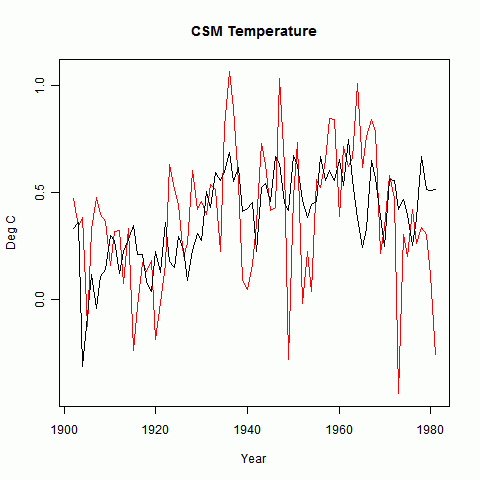
Fig 2 shows the full reconstruction. It mainly shows that the selected group came out somewhat higher, and the full proxy set is very noisy.



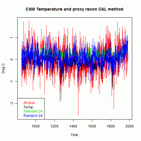
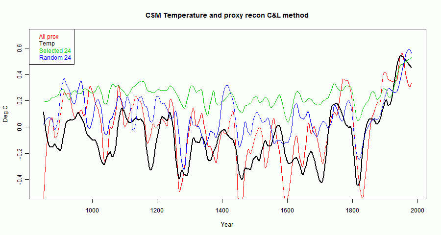
Fig 3 shows the reconstruction, but using Roman's smoother. It makes things clearer. The unscreened versions seem relatively unbiased but noisy. The screened version looks rather like Roman's CPS version, and has slightly smaller MSE (0.17).



I'll post the code tomorrow. This post is technically somewhat interim - I want to explore the effect of weighting according to regression uncertainty.

Update - code is here