Tests and results from TempLS v4 global temperature program.

I have been writing a series of articles leading up to the release of V4 of the prgram TempLS, which I run on the monthly data from GHCN (land) and ERSST V5. The stimulus for the new version was the release of GHCN V4. I use the program to compare with the major indices, which are basically GISS, NOAA, HADCRUT and BEST. I'll make comparisons of the TempLS output with those indices here.

I have been developing different integration methods, with the basic idea is that the agreement between a number of good methods with different basis is a guide to the amount of uncertainty that is due to method. I think it is quite small, and I will show comparative graphs. The key thing is that the different methods within TempLS agree with each other better than the indices agree among themselves.

One of the methods I have been exploring is the use of Spherical Harmonics (SH). This is not so much an integration method as an enhancement, and is so treated in TempLS V4. So the agreement between enhanced but otherwise inferior methods, and the better methods that are not enhanced, is further corroboration of the convergence of integration methodology.

I will illustrate all this with an active graph, of the kind I have been using for the index results themselves. You can, with mouse, change scales, translate axes, choose various subsets to plot, and also smoothe. An added facility here is that you can switch to difference plots in any combination you choose. I will at some stage post a facility like that for WebGL for doing this.

The post will be long, so I start with a table of contents.

Table of contents

• Brief summary of methods
• Active plot of results
• Comparison of methods.
• Methods in the context of indices and their variability
• Effect of enhancement
• Conclusion

Brief summary of methods

Some recent articles are here, here and here, with links to earlier. The methods I'll list are

• No weighting - the simple average of stations reporting in each month is used. This is a very poor method, but of interest here because it becomes quite serviceable after SH enhancement.
• Simple grid. This is the traditional method, where the temperature anomalies within each cell of, say, a lat/lon 2° grid, are averaged, and the global is then the area-weighted average of the cells that have results. Area-weighting relates to the shrinking of area of cells near the poles. It is used by HADCRUT; the paper of Cowtan and Way showed that the effect of accounting for cells without data gave an important correction to trends. I do not now use lat/lon grids, but rather a cubed sphere, or other platonic solid based grid. The alternative is usually icosahedron. In each case I use mappings to make the cells of almost uniform area.
• Grid with infill. This assigns to empty cells a value based on neighbors. Most recently, I do this by solving a Laplace equation, with the known cell values as boundary condition. That sounds complex, but the simple Southwell relaxation method, , which initially guesses the unknown cells, and then replaces with the average of neighbors until convergence, is quite adequate.
• Irregular triangular mesh. This has been my workhorse; it is basically finite element quadrature, with linear interpolation within triangles with stations as vertices. I have thought of it as my best method.
• First order LOESS. This sets up a regular array of nodes (icosahedral), and assigns values to them based on local first order weighted regression with a typically 20 of the nearest stations. The regular array is then simply averaged. I think this is a rival for the best method.

Active plot of results

The idea of active plotting is described here, and my regular example is the monthly plot of indices here. The active plot for this post is here, with details below:

Description and code of TempLS V4 global temperature program.

It's now time to post the code for TempLS V4. I know that it is a day when many folks who really want to get their message read put it out to the world. I didn't want to steal anyone's thunder; the week just didn't have enough days. I've been writing background articles leading up to the release of V4 of TempLS; here are the links:
ideas about spatial integration
icosahedral grid with equal area mapping
documentation system
details of new methods
tests
math methods

TempLS is a code written in R, dating back to about 2010 - there is a summary of its history up to V3 here. The release post (Aug 2010) for V2 is here; Ver 3 was rolled out in three parts, of which the last, here, links to the earlier parts.

Release of V4 is, as I mentioned in the documentation post, complicated by the fact that I use extensively a library of R functions that I keep, and will need to include. But I hope the documentation will also help; I'll be relying on it for this release.

The release is in three zip files, LScode.zip, Moyhupack.zip and LSdata.zip

• There is a file of code and some internal data - LScode.zip. To run it, you should extract it in an empty directory; it will create six subdirectories (x,g,i,l,m,n). The R file to run it is LS_wt.r, explained below. This zip file is about 98 Kb.
• As mentioned before, the code now has a lot of generic functions embedded from my general library. There is a documentation system explained at that link, which I also used for the functions of TempLS, below. This zip file includes a list Moyhupack.rda. This you can attach, R style, as a package, which has advantages. The functions from it are also on a file Moyhupack.r, which you can just source() into your environment. It has a lot of functions with short names, most of which you won't want to know about, so there is potential for naming clashes. Finally, there is a documentation file Moyhupack.html. If there is interest, I will write more about the library. I think it does have useful things for math programming. The zipfile is about 800 Kb Moyhupack.zip
• Finally, there is a set of data. The main one is a recent version of GHCN V4 unadjusted TAVG, named ghcnv.dat. There is also the inventory file that came with it, called ghcnv.inv. The SST data is from ERSST V5; it is part processed in TempLS style and in a directory called x. Note that the code zipfile also created an x directory, with just one list, which would overwrite this larger version if unzipped later. This is a big file - about 54 Mb (mainly GHCN). LSdata.zip

The math task and code structure

As before (V3 and earlier), the code is divided into four parts, The code starts with a text version of GHCN V4, and goes looking for a NetCDF version of ERSST V5, if needed. It assembles all this data into 12 (month) arrays of station temperature (rows) vs year (cols). ERSST grid cells count as stations. Missing values are marked with NA. The objective is to fit the model
T=L+G
where T is the station temperature, L the time-invariant normal, and G the space-invariant global anomaly. The fitting requires integration, which comes down to a weighted sum of the data. The third section of the code uses the data about stations reporting, but not the temperatures, to work out weights for integration by various methods. This can be by far the most time-consuming part of the code, alleviated greatly by the use of past calculated weights where the list of stations reporting hasn't changed.

The fourth section is where the fitting is done, via a brief iteration (few seconds) to get convergent values of L and G, which is the main output. It is also where the optional Spherical Harmonics enhancement is done.

Code details.

The code is now almost entirely done as function calls. I call the main file LS_wt.r, which calls functions from LS_fns.r. These are documented below. The main sequence functions (the four parts) are

• SortLandData() handles land data
• SortSSTData() handles ERSST5 data.
• DeriveWeights() calculates weights from the x array of the previous parts
• FitGlobal() does the iterative fitting to produce L and G.

There are three lists of data that are switched in and out as needed; they are:

• I the inventory data, which governs the dimensions of later data matrices. It is updated in a controlled way by newinv() on LSinv.rds
  
• 
  J is to describe the results in SortLandData and SortSSTData - assembling x. On LS.rds
• K is for the method-dependent data in DeriveWeights and FitGlobal, including the main result, K$G.

The 12 (month) temperature files are stored in directory x. The 12 weight files are stored in directories, one for each method
("g","i","m","n","l") for ("grid","infilled","mesh","none","loess"). Since the K data is method dependent, a separate version is stored on each directory as LS.rds.

Code sequence

The main code is:

source("LS_fns.r") if(!exists("job"))job="UEMO" print(paste("Starting",job,Sys.time())) i=vsplit(job,"") kind=tolower(i) kinds=c("g","i","m","n","l") RDS=pc(kind[3],"/LS.rds") K=readRDS(RDS) # I is inv list, J is list about x, K is list for method kind (w) K$edition=I$edition K$kind=kind; K$job=job; do=i!=kind wix=pc(kind[3],"/") # info about w tm=timex(0); tx=unlist(tm); t0=Sys.time(); yr=c(1900,tx[1]+(tx[2]>1)-1); yrs=yr[1]:yr[2]; # you can change these ny=diff(yr)+1 saveR(K) if(do[1])SortLandData() if(do[2])SortSSTData() if(do[3])DeriveWeights() if(do[4])K=FitGlobal()

As previously, the user supplies a job string of four characters. They are uppercase if that code section is to be performed. A typical value is job="UEMO". At the moment there aren't realistic alternatives for "UE", which is unadjusted GHCN V4 and ERSST V5. M stands for mesh method, but could be any of ("G","I","M","N","L"). "O" just means perform last section; "P" means go on to produce graphics with another program.

A second control variable that can be set is nSH=4, say. It induces the spherical harmonics enhancement, and the value sets the order, using (nSH+1)^2 functions. Going past 10 or so is risky for stability (and time-consuming).

The third control is called recalc. It lets you override the system of using stored values of weights when the stations reporting in a given month is unchanged. This saves time, but it can happen that you suspect the stored data is wrong, for some reason. Something might have gone wrong, or the inventory might have changed. The default setting is FALSE, or 0, but if you want it to not use stored data, set recalc to 1. There is also a setting that I find useful, recalc=2, which recalculates only the most recent year. This takes very little time, but will check if the code is currently working for that method option. Otherwise if it uses entirely stored data, it could take some time to find errors.

So the actual code here just brings in K, which also acts as a record of what was done. It stores some information and puts K back on disk. The other stuff just makes some time information for use in the main sequence. Note that the last step outputs K. This is where the results are (K$G and K$L).

Documentation of functions

Remember there are a lot of generic functions on the Moyhu package. The functions here are those specific to TempLS.

GISS March global up 0.21°C from February.

The GISS V3 land/ocean temperature anomaly rose 0.21°C in March. The anomaly average was 1.11°C, up from December 0.90°C. It compared with a 0.208°C rise in TempLS V3 mesh. Jim Hansen's detailed report is here. So far, April is looking warm too.

I think that now that TempLS and GISS are using GHCN V4, the agreement will be even better than in the past, as in this month. There extra coverage does make a difference. The earlier NCEP/NCAR average also agreed very well (0.19° rise). It was the third highest March in the record, just behind 2017.

The overall pattern was similar to that in TempLS. Huge warm spots in Siberia and NW N America/Arctic. Cool spots in NE USA through Labrador to Greenland, and Arabia through N India. Warm in Australia and S Africa.

As usual here, I will compare the GISS and previous TempLS plots below the jump.

The math basis for the TempLS V4 global temperature program.

This is, I hope, the last of the preparatory posts before I post the code and description of TempLS V4. Earlier posts were on ideas about spatial integration, an icosahedral grid with equal area mapping for a new method, the documentation system that I'll be using, details of new methods, tests, and some math methods that I'll be using and referring to.

The math basis is similar to what I described back in 2010 for V2, and in the guide to V3, still the most complete reference. The statistical model for temperature for a given month (Jan-Dec) is:

T = L + G, where T is measured temperature, L is a time-invariant offset for stations, and G a space-invariant global average temperature. In more detail, using my index notation, with s for station, y for year, and m for month, it is

T_smy = I_yL_sm + I_sG_my

The I's are added for consistency of indexing; they denote arrays of 1's.

A change in V4 is that the analysis is done separately over months, to avoid over large arrays in RAM. That simplifies the analysis; the subscript m can be dropped. Another change is more subtle. The model fitting should be by area and time, ie by minimising the integral of squares

In earlier versions I discretised the variables jointly, giving a weighted sum

w_(sy)(T_sy-I_yL_s + I_sG_y)²

In fitting, this gave a matrix which was symmetric positive definite, which seemed natural and good. But it means that if you choose the weights to be right for the spatial integration, they can't be controlled for the time integration, so locally, they vary over years, which isn't really wanted. For the methods I used in v3, the weights were all positive, and of reasonably uniform size, so it didn't really matter. But in V4 I use methods which are higher order, in taking account of derivatives. Sometimes, for good reason, the weights can be negative. Now for spatial integration, they add to the area, so that is still OK. But for time integration, there might be significant cancellation, with a sum that is near zero, or even negative. It doesn't often happen, but since you have to divide by the sum of weights to get a time average, it is bad.

Revised weighting - Gauss Seidel iteration

The previous equations, derived from the sum squares, were

w(s)y(Tsy-IyLs - IsGy)=0		(1a)
ws(y)(Tsy-IyLs - IsGy)=0		(2a)

To get even time weighting in (1a), I use a weighting J_(s)y, which is 1 where there is a reading, and 0 where there isn't (where w also had zeroes).

J(s)y(Tsy-IyLs - IsGy)=0		(1b)
ws(y)(Tsy-IyLs - IsGy)=0		(2b)

This can be written in part-solved form as

J(s)yIyLs = J(s)y(Tsy - IsGy)=0		(1)
ws(y)IsGy = ws(y)(Tsy-IyLs)=0		(2)

The first just says that L is the time average of T-G where observed, since its multiplier is just the set of row sums of J, which is the number of years of data for each station. The second then is just the area average of T corrected for L (the anomaly, whne L has converged). Suitably normalised, the multiplier of G is 1. Starting with G=0, this gives "naive averaging", with L just the overall time mean at station s. As I wrote here, this gives a bad result, which is why the main methods insist on averaging over a fixed time period (eg 1961-90). But that then leaves the problem of stations that do not have data there, which this method avoids.

So the first equation is solved, and the L used to estimate G, which is then used to correct, L, and so on iterating. The reason that iteration works is that the equations are weakly coupled. Eq (1) almost fixes L, with variations in G having only a small effect. Conversely Eq (2) almost fixes G, not very sensitive to local variations in L. There is an exception - if you add a constant value to G, it will cause the L's to drop by a similar constant amount.

So that is the iteration sequence, which can be characterised as block Gauss-Seidel. Start with a guessed value for G. Solve (1) for L, then solve (2) for an updated value of G. For GHCNV4, as used here, this converged gaining at least one significant figure per iteration, so four or five steps are sufficient. In practice, I now start with a previous estimate of G, which converges even faster. But in any case, the step takes only a few seconds. At each step, G is normalised to have mean zero between 1961 and 1990 (for each month), to deal with the ambiguity about exchanging a constant value with L.

Program structure

As before, TempLS has four blocks of code, now expressed as functions:

• SortLandData
• SortSSTData
• DeriveWeights
• FitGlobal

The first two are just housekeeping, ending with x_sy, the array of monthly temperatures. The third derives the corresponding spatial integration weight matrix w_sy by one of five methods described here. The fourth, FitGlobal(), performs the iteration described above. The result are the parameters G and L, of which G is the desired global temperature anomaly, which I publish every month.

For the more accurate methods, DeriveWeights is the most time consuming step; a full meshing can take an hour, and LOESS takes ten minutes or so to do the full record since 1900. But the weights depend only on the stations reporting, not what they report, and for most of those years this doesn't change. So I store weights and reuse them unless there is evidence of change in the list of stations that reported that year. This brings the compute time back to a few seconds.

In V3, I had a separate method based on Spherical Harmonics. As described here, I now treat this as an enhancement of any method of integration. In V3, it was in effect an enhancement of the very crude method of unweighted averaging over space. It actually worked well. In V4 it is implemented, optionally, at the start of FixGlobal(). The weights from part 3 are modified in a quite general way to implement the enhancement, with results described in the post on tests. I think it is of interest that as a separate integration principle, it yields results very similar to the more accurate (higher order) integration methods. But I don't think it will have a place in routine usage. It takes time, although I now have a much faster method, and it does not give much benefit if the more accurate methods are used. So why not just use them?

Some math used in TempLS - index notation and sparse matrices.

Index notation for arrays, and the summation convention

Index notation for arrays became popular with the tensor calculus, partly because it also elegantly embraced the concepts of contravariance and covariance. It is sometimes called the Einstein notation. I'm not using the tensor aspect here, so no superscripts. Arrays, including vectors, are simply represented by writing down their coefficients with subscripts, with the understanding that those vary over a known range. There is no attempt to visualise them geometrically. The coefficients, like arrays, can be added if the subscripts match in range, and be multiplied by scalars or pother subscripted arrays.

But the core of the system is the summation convention, also named after Einstein. It expresses the idea of inner product, which is what distinguishes matrices from just vectors. If an index is repeated in a term, it implies summation over the range of that index. Some familiar cases:

aibj	is the outer product of two vectors, functioning as a 2-index array, or matrix, but
aibi	is the inner product, with a single number (scalar) result. i is referred to as a dummy variable, because it won't be referenced again.
aijbj	is a matrix right multiplied by a vector. The result is a vector, indexed with i
aijbi	would be left multiplied. But that terminology isn't needed; the indices say it all.
ajj	is the trace of matrix A
aijbjk	is the matrix product A*B, indices i and k.
aijbjkck	is the product A*B*c, a vector, index i

You can exempt an index from the repetition count with braces, so a_(i)b_i is not summed. The multiplication is real, so it is as if A was a diagonal matrix. It often appears as a kernel, as in a_(i)b_ic_i, which would be a quadratic form with diagonal matrix A as kernel.

I use a special notation I_j or I_jk for an array consisting entirely of 1's.

I have used this notation at least since introducing V2 of TempLS, but I'll be making more extensive use of it with V4. A feature is that once you have written down an index version of what you want to do, it maps directly onto R coding.

Sparse matrices

Often the indices have a small range, as over space dimensions. But sometimes the range is large. Most integration methods in TempLS involve mapping from one large set, like stations, to another, like grid cells. At some point there will be a matrix involving those two indices. In V4 we might have 30,000 stations, and 10,000 cells. You would not want to enter such a matrix into RAM.

The saving grace is that most nodes have no interaction with most cells. As with partial differential equations in maths, the relations are local. Most terms are zero, a sparse matrix. So it is possible to enter the non-zero terms, but you also have to say where they are in the matrix. I just list the N nonzero terms in a vector and in a Nx2 matrix, I list first the row and then the column of each term.

The key issue again is matrix-vector multiplication y=A*b. This is what can take a set of numbers over stations to one over grids. In a language like C, with this structure, the algorithm is simple. You go through that list, take each a_pq, multiply by b_q, and put the result in y_p. But that is a lot of operations, and in an interpreted language like R, they carry too much overhead. It would be possible to stretch out the terms of b to match a, so the multiplication could be between vectors. But they can't be added into the result vector in one operation, because several numbers would have to be added into one location. I use an algorithm that sorts the indices of a into subsets that do correspond to a unique location, so the multiplication can be reduced to a small number of vector operations.

Use in TempLS

I have written. for example here and very recently here about ways in which spatial integration is done in TempLS, and why. Integration is a linear operation on a set T_s of measured temperatures, or anomalies, and so the result can be represented as a weighted sum, w_sT_s. For each method, the first task of TempLS is to calculate those weights.

I'll go through the basic arithmetic of simple gridding from this viewpoint. To integrate directly, you work out which cells of the grid the stations belong to, calculated an average for each cell, and then multiply those by the areas of each cell and add. It's fairly simple to program, but I'll describe it in sparse matrix terms, because more complex cases have a similar structure.

The key matrix being formed is the incidence matrix In over indices g for grid (rows) and s for stations (columns). This is zero, except where station s is in cell g, when it has a 1. So the action of summing station data x in cells is the product In_gsx_s. The sum has to be divided by the count, which in matrix terms is the product In_gsI_s. The result then has to be multiplied by the grid areas a_g and added. Overall

Integral over earth = a_g (I_tIn_(g)t)^-1 In_gs x_s

The result has no indices, so all must be paired. Note the appearance of a bracketed (g) in the denominator. The repetition of separate station indices s and t indicates two separate summations.

Forming the index set for the sparse matrix is usually simple. Here the right column just numbers the stations, starting from 1. The left column just contains the cell number that that station is in.

That was reasoned starting from known x. To calculate the weights w, x must be removed, and the linear algebra started from the other end, with matrices transposed. Transposing a sparse matrix is trivial - just swap the columns of the index.

I'll go through the algebra for more complex cases in a future post, probably in conjunction with the code. But here is a table showing how the basic structure repeats. These are the various integration algorithms in index notation.

No weighting	(ItIt)-1Isxs
Simple grid	ag (ItIn(g)t)-1 Ings xs
Triangle mesh	ag Ings xs	a = areas of triangles
Loess order 0	Ip (ItW(p)t)-1 Wps xs	W is a function (with cutoff) of distance between station s and nearby node p.
Loess order 1	ypj (ztjztkW(p)t)-1 Wpszsk xs	zsk are the station of station s; ypj are the coordinates of node p.

Testing integration methods in TempLS V4.

I posted yesterday about some new methods and changes in integration in TempLS V4, explaining how the task is central to the formation of global temperature anomaly averages. Today I will show the results of testing the methods. We can't test to see if actual data gives the right result, because we don't know that result. So tests are of two types

• Testing integration of functions whose average is known. Values of those functions replace the observed temperatures in the process, with the same station locations and missing values.
• Comparing different methods, to see if some converge on a common answer, and which do not.

I tested six methods. They are, in order (approx) of ascending merit

• Simple average of stations with no area weighting.
• Simple gridding, with cells without data simply omitted. The grid is cubed sphere with faces divided into 24x24, with a total of 3456 cells. Cell area is about 25000 sq km, or 275 km edge.
• Zero order LOESS method, as described in last post. Zero order is just a local weighted average.
• Gridding with infill. Empty cells acquire data from neighboring stations by solving a diffusion equation, as briefly described in the last post.
• First order LOESS, in which values on a grid of nodes are calculated by local linear regression
• Finite element style integration on a triangular mesh with observation points at the vertices.

I said the order was approximate; there is some indication that full LOESS may be even slightly better than mesh. I also tested the effect of using spherical harmonics fits for enhancement, as described here. This option is now available in TempLS V4. The parameter nSH is a measure of the number of periods around the Earth - see here for pictures. For each level of nSH, there are (nSH+1)^2 functions.

Testing known functions

An intuitively appealing is simply latitude. Using just the latitude of stations when they report, in January 2011, what does the process give for the average latitude of the Earth. It should of course be zero.

	nSH=0	nSH=2	nSH=4	nSH=8	nSH=12
No weighting	26.6295	-0.0393	-0.0603	0.0479	1.9308
Grid no infill	0.5095	0.0806	-0.0121	-0.035	-0.0197
LOESS order 0	0.022	-0.0342	-0.0438	-0.0342	-0.0216
Grid diffuse	-0.0432	-0.0466	-0.037	-0.0267	-0.0175
LOESS order 1	-0.023	-0.0231	-0.0252	-0.0223	-0.0182
Mesh FEM	-0.0209	-0.022	-0.0218	-0.0177	-0.0129

The case with no weighting gives a very bad result. A very large number of GHCN V4 stations are in the US, between lat 30° and 49°, and that pulls the average right up. Grid with no infill also errs on the N side. The reason here is that there are many cells in the Antarctic and near without data. Omitting them treats them as if they had average latitude (about 0), whereas of course they should be large negative. The effect is to return a positive average. The other methods work well, because they are not subject to this bias. They have errors of local interpolation, which add to very little. The poor methods improve spectacularly with spherical harmonic (SH) enhancement. This does not fix the biased sampling, but it corrects the latitude disparity that interacts with it. Deducting the non-constant spherical harmonics, which are known to have average zero, leaves a residual with is not particularly biased by hemisphere. The no weighting case is bad again at high order SH. The reason is that the fitting is done with that method if integration, which becomes unreliable for higher order functions. I'll say more about that in the next section.

Testing spherical harmonics.

Latitude is a limited test. SH's offer a set of functions with far more modes of variation, but testing them all would return a confusing scatter of results. There is one summary statistic which I calculate that I think is very helpful. When you fit SH Fourier style, it is actually a regression, involving the inverse of the matrix of integrals of products of SH. This is supposed to be the identity matrix, but because of approximate integrations, the SH are not exactly orthogonal. The important number indicating deviation from unit is the condition number, or ratio of max to min eigenvalues. When it gets too low, the inversion fails, as does the fitting. That is what was happening to unweighted averaging with nSH=12. So I calculated the minimum eigenvalue of that matrix (max remains at 1). Here is a table:

	nSH=2	nSH=4	nSH=8	nSH=12
No weighting	0.0703	0.0205	-0.8361	-0.9992
Grid no infill	0.7893	0.631	0.4354	0.1888
LOESS order 0	0.9501	0.8298	0.4593	0.1834
Grid diffuse	0.9694	0.9013	0.6026	0.2588
LOESS order 1	0.988	0.9503	0.6905	0.3037
Mesh FEM	0.9875	0.9418	0.6677	0.3204

Close to 1 is good. There is a fairly clear ranking of merit, with full LOESS just pipping mesh. No weighting is never good, and completely falls apart with high nSH, being not even positive definite. All methods are down quite a lot at nSH=12, although a minimum of 0.3 say is not a major problem for inversion. These values are for January 2011, but it is a robust statistic, varying little from year to year. Here is the comparison over years for the nSH=8 level:

	2011	2012	2013	2014	2015	2016	2017	2018	2019
No weighting	-0.8361	-0.759	-0.2471	-0.2119	-0.0423	-0.0104	0.01	0.0167	0.0199
Grid no infill	0.4354	0.465	0.4481	0.4129	0.4493	0.4237	0.4394	0.4325	0.4436
LOESS order 0	0.4593	0.4972	0.4742	0.4477	0.4791	0.4472	0.4734	0.4697	0.4764
Grid diffuse	0.6026	0.6207	0.6102	0.5741	0.6132	0.5929	0.6127	0.608	0.6095
LOESS order 1	0.6905	0.711	0.6965	0.6762	0.6912	0.6832	0.6903	0.6927	0.6944
Mesh FEM	0.6677	0.6663	0.6703	0.6636	0.6627	0.6737	0.6741	0.6772	0.6626

Test of global average of real anomalies.

For consistency, I have used real temperature data with the station normals calculated by the mesh method. It would not matter which method was used, as long as it is consistent. Here are January results over years with no SH enhancement:

	2011	2012	2013	2014	2015	2016	2017	2018	2019
No weighting	-0.1565	1.2277	0.5341	0.3475	1.0401	0.7213	0.9881	0.8065	0.8183
Grid no infill	0.3254	0.2995	0.4834	0.5251	0.6729	0.9464	0.8194	0.6127	0.7443
LOESS order 0	0.366	0.2988	0.5224	0.5665	0.6649	1.0036	0.8499	0.619	0.7425
Grid diffuse	0.3674	0.2919	0.5113	0.5443	0.6495	0.9802	0.8283	0.6186	0.7111
LOESS order 1	0.3706	0.2994	0.5057	0.5397	0.6429	0.9932	0.8281	0.6209	0.7112
Mesh FEM	0.3779	0.2862	0.5051	0.517	0.6474	0.9969	0.8088	0.6178	0.7017

The best methods are really very close, generally within a range of about 0.02. Even simple grid (with cubed sphere) is not that different. But no weighting is bad. The effects of SH enhancement are variable. I'll show them for January 2018:

	nSH=0	nSH=2	nSH=4	nSH=8	nSH=12
No weighting	0.8065	0.8842	0.5687	0.5633	1.4847
Grid no infill	0.6127	0.6253	0.6077	0.6165	0.6139
LOESS order 0	0.619	0.6196	0.6138	0.6224	0.6152
Grid diffuse	0.6186	0.6194	0.6191	0.6241	0.6237
LOESS order 1	0.6209	0.621	0.6198	0.6225	0.619
Mesh FEM	0.6178	0.6182	0.618	0.6206	0.6147

The better methods do not change much, but converge a little more, and are joined by the lesser methods. This overall convergence based on the separate principles of discretisation type (mesh, grid etc) and SH enhancement is very encouraging. Even no weighting becomes respectable up to nSH=8, but then falls away again as the high order fitting fails. I'll show in a future post the comparison results of the different methods for the whole time series. There are some earlier comparisons here, which ran very well back to 1957, but were then troubled by lack of Antarctic data. I think LOESS will perform well here.

New methods of integration in TempLS V4 for global temperature.

Background

TempLS is a program that takes the extensive data of surface temperature measurements and derives a global average of temperature anomaly for each month over time. It also produces maps of temperature anomaly distribution. The basic operation that enables this is spatial integration. As with so much in science and life, for Earth's temperature we rely on samples - it's all we have. To get the whole Earth picture, it is necessary to interpolate between samples. Integration is the process for doing that, and then adding up all the results. The average is the integral divided by the area.

The worst way of getting an average is just to add all the station results and divide by the total. It's bad because the stations are unevenly distributed, so the result reflects the regions where stations are dense. This generally means the USA. Some kind of area weighting is needed so that large areas with sparse readings are properly represented. Early versions of TempLS used the common method of gridding based on latitude/longitude. The default method of spatial integration is to form a function which can be integrated, and which conforms in some way to the data. In gridding, that function is constant within each cell, and equal to the average of the cell data. But there is the problem of cells with no data...

Since V2, 2011 at least, TempLS has used unstructured mesh as its favored procedure. It is basically finite element integration. The mesh is the convex hull of the measurement points in space, and the area weight is just the area of triangles contacting each node. For over seven years now I have reported average temperature based on the mesh method (preferred) and grid, for compatibility with Hadcrut and NOAA.

Early in the life of V3, some new methods were added, discussed here. The problem of cells with missing data can be solved in various ways - I used a somewhat ad-hoc but effective method I called diffusion. It works best with grids that are better than lat/lon. I also used a method based on spherical harmonics, with least squares fitting. As described here, I now think this should be seen as an enhancement which can be applied to any method. It is spectacularly effective with the otherwise poor method of simple averaging; with better methods like mesh or diffusion, there is much less room to improve.

So why look for new methods?

We don't have a quantitative test for how good a method is applied to a temperature field. The best confirmation is that the methods are relatively stable as parameters (eg grid size) are varied, and that they agree with each other. We have two fairly independent methods, or three if you count SH enhancement. They do agree well, but it would be good to have another as well.

V4 changes.

V4 does introduce a new method, which I will describe. But first some more mundane changes:

• Grid - V4 no longer uses lat/lon grids, but rather grids based on platonic solids. Currently most used is the cubed sphere, with ambitions to use hexagons. All these grids work very well.
• Spherical Harmonics - is no longer a separate method, but an enhancement available for any method. It's good to have, but adds computer time, and since it doesn't much enhance the better methods, it can be better to use them directly.
• I have upgraded the diffusion method so that it now solves a diffusion equation (partial differential) for the regions without cell data. The process is very simple - Southwell relaxation, from the pen and paper era, when computer was a job title. You iterate replacing unknown values by an average of neighbors.

The LOESS method

The new method uses local regression - the basis of LOESS smoothing. Other descriptive words might be meshless methods and radial basis functions. The idea is that instead of integrating the irregular pattern of stations, you find a set of regularly spaced points that can be integrated. In fact, using an icosahedron, you can find points so evenly spaced that the integral is just a simple average. To estimate the temperatures at these points, weighted regression is applied to a set of nearby measurements. The regression is weighted by closeness; I use an exponential decay based on Hansen's 1200 km for loss of correlation. But I also restrict to the 20 closest points, usually well within that limit.

The regression can be relative to a constant (weighted mean) or linear. The downside of constant is that there may be a trend, and the sample points might cluster on one side of the trend, giving a biased result. Linear fitting counters that bias.

I'll show test results in the nest post. I think the LOESS method is at least as accurate as the mesh method, which is to say, very accurate indeed. And of course, it agrees well. It is flexible, in that where data is sparse, it just accepts data from further afield, which is the best that can be done. You could think of a grid method as similarly estimating the central values, which can then be integrated. The grid method, though, artificially cuts off data that it wall accept at the cell boundary.

The LOESS method also gives a good alternative method of visualisation. My preferred WebGL requires triangles with values supplied at corners, when GL will shade the interior accordingly. I have used that with convex hull mesh (eg here), but when triangles get large, it produces some artifices. Using the underlying icosahedral mesh of LOESS has uniformly sized triangles. Of course, this is in a way smoothing over the problem of sparse data. But at least it does it in the best possible way.

Here is a WebGL plot of June 2019 (changed later) temperature anomaly, done the LOESS way. As usual, there are checkboxes you can use to hide the mesh overlay, or the colors, or even the map. More on the facility and its use here.

You can contrast the effect of the LOESS smoothing with the unstructured mesh representation here. Both present unadjusted GHCN V4, which clearly has a lot of noise, especially in the USA, where quantity seems to degrade quality. None of this detracts from global integration, which smooths far more than even LOESS. I think that which it is occasionally of interest to see the detail with the mesh, the LOESS plot is more informative. The detail of mesh had been useful in GHCN V3 for spotting irregularities, but in the US at least, they are so common that the utility fades. In much of the rest of the world, even Canada, coherence is much better.

March global surface TempLS (with GHCN V4) up 0.208°C from February.

This is the first month of full use of the new GHCN V4 land temperature data (unadjusted). It's also using the new version V4 of TempLS, which I will post and describe shortly. The usual report is here, showing the map, the breakdown in regions, and the stations reporting. The detailed WebGL plot is here, and it is a good way of capturing the extra detail available in GHCN V4. It also shows the greater patchiness of the stations, which is partly countered by the greater numbers. It is particularly bad in the US, with so many volunteer stations.

I'm still getting a feel for when is the best time to post. I used to wait until the main countries reported, but with V4 it isn't done by country, and even after four or five days there are a lot of stations with apparently good coverage. But there are still many more stations to come, so there is still the possibility of a late drift. We'll see.

The TempLS mesh anomaly (1961-90 base) was 0.964deg;C in March vs 0.756°C in February. As with the NCEP/NCAR reanalysis index, that makes it a very warm month, especially as February was already warmer than January, and even more so than last November. It was the warmest month since March 2017 (which was just 0.01°C warmer), and the third warmest March in the record.

As with the reanalysis the main features were big warmer areas in Siberia and Alaska/NW Canada, joining up over the adjacent Arctic ice layer. The warmth extended into Europe, especially the East. It was generally cool in the US, and in a belt from Tibet to Egypt.
Here is the temperature map. Southern Africa and Australia were quite warm.



And here is the map of stations reporting:

New TempLS v4 preamble - a documentation system.

Background

I'm gearing up to release TempLS V4. I have been working on this (and am now using it) to manage the extra demands of GHCN V4. A complication is that I now use a lot of my own library functions in R. For V3 I could replace them, but now they are too heavily embedded. So I'll hneed to supply the library as well. This works like an R package, but has a different documentation system, which I'll now describe. I think it is better, and I'll use it for the code of TempLS V4 as well. There is an example of the system at the end, and following that, a zipfile with all the entities involved, including the R code.

Motivation for a different system

I write a lot of R code, and I have a set of functions that I currently load in to be part of the working environment. I also have a library of Javascript functions that I import. I need a scheme where these are kept in some organising system with associated documentation. I would like this to be very easily edited, and then generated as HTML for easy reference.

The classic R way of doing this is to create and attach a package. This is a list of parsed functions that are not in the working environment, but sit on the search path at a lower level. That means that they don't overwrite existing names, but those names in the environment might block access to the package functions. R has a system for documenting using an associated .rd file. This has a Latex-like language, and a lot of structure associated with it.

I want to use the attach system, but I find the requirements of the package documentation onerous. They are meant to support packages for general release, but I am the only user here. I want a closer association between documentation and code, and a faster system of updating the HTML.

A system designed for this is Doxygen. This has an implementation as the R package roxygen2, based on embedded comments. This again works through .rd files which it turns into pdf. This is more cumbersome than I would like. I also want to use the system for objects other than functions, which can be included in the package.

So I have created a set of R programs which work through a list of lists, each specifying a function, or perhaps some other object that I would like to see in a package. I call that master list an object. It isn't useful in itself, but can easily be converted into a package that could be attached. But it can also easily generate the HTML documentation with appropriate layout. But a further facility is that it can generate a text file in which the documentation and code are listed together and can be edited, and then mapped back into the object form.

Although I adopted the scheme for its flexibility when I make frequent changes, I think it is now justified by the better active HTML reference page. Not only does it have various linked indexes, but you can choose to display the code next to the documentation. And since the code is placed there at the same time as it is entered into the package, it is guaranteed to be current, even if the manual editing of the description may lag.

The material for the object comes generally from collections of R functions used in a program environment, so there needs to be a scheme to import this into an object. It is desirable to be able to map back, because writing and debugging code is best done in the native form. Since the object contains a lot of text as well as functions, it is important to have a merge facility, so that updated functions can be imported while retaining the documentation.

This all works, and can be extended to other languages, although I'll refer to it as R code here.. I use it for Javascript. There isn't the exact equivalent of an attachable package, but code can still be output in a usable form. Importing from code works in much the same way, since it relies on functions being delimited by braces. So it could be used for C and similar languages as well. The main thing is that the html and text forms are useful in the same ways.

Here is a diagram of the various forms and transitions:

		Pack
		⇑↓
Text	⇌	Object	⇌	Code
		⇓
		html

And here are more details about the entities. The naming convention will be that there is a stem name, and the files will be called stem.rda, stem.txt, stem.html The results can be accessed directly in the namespace, as well as returned.

March NCEP/NCAR global surface anomaly up 0.19°C from February

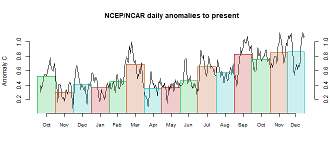
The Moyhu NCEP/NCAR index rose from 0.393°C in February to 0.582°C in March, on a 1994-2013 anomaly base. Cumulatively, that is a rise of 0.29°C from January, and is 0.4°C warmer than last November. That makes it the warmest month since the peak of the 2016 El Niño, Feb/March 2016, and so is the second warmest March in the record.. It was warm through the month, but most at the beginning and end.

The US was still cool, as was E Canada. But the NW of N America was very warm, as with the Arctic ocean above. There was warmth right through Siberia, into most of Europe and down to Kazakhstan and N China. Below that, a belt of cool from Tibet to the Sahara. Mixed, with nothing very pronounced, in the Southern Hemisphere. However, although Australia looks only moderately warm on the map, the BoM says it was the warmest March on record.

The BoM ENSO Outlook is upgraded to Alert - "This means the chance of El Niño forming from autumn is around 70%; triple the normal likelihood" Remember, that is SH autumn - ie now. .