Pausebusting NOAA

In previous posts here, here and here, I have been discussing issues in infilling cells in the HADCRUT 4 dataset, following a new much-discussed paper by Kevin Cowtan and Robert Way in QJRoyMetSoc. They used satellite data and kriging to extend the data; I looked at a much simpler approach of infilling with latitude averages from the same data (rather than the implicit infilling with global average). I found that it gave rather similar results, although with more limited effect.

Now I want to try it with the similar NOAA gridded data set which is used for their index. They give a detailed description at this download site. It is a similar 5°x5° grid, so the same analysis should work.

I show below first plots of both HADCRUT 4 and NOAA coverage. NOAA has greatly fewer gaps, but also fairly extensive omissions near the poles. Then I show the latitude breakdowns, with seasons. I have included the C&W and UAH plots for comparison.

Coverage plots

This is an active plot - you can choose dataset and view. It counts data in each cell/month from 1979 to 2012. Red is for no data, cyan is complete, and there is shading for intermittent data.

NOAA N NOAA S HAD 4 N HAD 4 S

NOAA coverage is more extensive than HADCRUT, with some odd inclusions (eg central Greenland) and omissions (S Pole). Still, I found using the latitude average method described in previous posts with smoothing parameter r=0.1, that I had to include an extra level of bands to get enough data for lat 85-90S.

Latitude average trends

This is a similar active plot to the one in the previous post. NOAA data replaces HADCRUT 4, and I have increased the width of those curves, since they are new. UAH and the C&W hybrid HADCRUT 4 result are included for comparison.

Annual DJF MAM JJA SON

(Update - again I made an error with latitude sign (the problem is that HADCRUT orders from N Pole, NOAA from S) So NOAA were reversed, Fixed now.)
The background stripes indicate the latitude bands; N pole is on the right. There's a faint red vertical marking multiples of 30°. In the centre is a little figure showing the global totals, on the same scale.

Here is a table of the global trends, 1997-2012 in C/decade:

Season	NOAA	NOAA Av	HADCRUT 4	HAD 4 Lat Av	UAH	C&W Hybrid
DJF	-0.0519	-0.0049	-0.0489	0.0097	0.0276	0.0536
MAM	0.0688	0.1123	0.066	0.1019	0.0639	0.1276
JJA	0.0629	0.0789	0.0892	0.0966	0.12	0.1187
SON	0.1084	0.1347	0.1081	0.1277	0.1575	0.1688
Annual	0.0485	0.0814	0.0539	0.0844	0.0936	0.1187

The results of NOAA and HADCRUT 4 are very similar, in effect on trend and in seasonal variation. Both show a substantial trend increase in trend over this period, as a result of simply using the appropriate latitude average to infill rather than the global.

Seasonal trends for infilled HADCRUT

I have been posting on ways of dealing with cells in the HADCRUT 4 surface temperature anomaly grid which have no data. This follows a new much-discussed paper by Kevin Cowtan and Robert Way in QJRoyMetSoc. They used satellite data and kriging to extend the data, particularly into polar regions. The result that created particular interest concerned trends in a recent period, 1997-2012, which has been characterised as a "pause", partly because HADCRUT showed little trend. C&W found that the trend was significantly greater with this extra care.

I have been discussing this, in posts here and here. In the second post, I showed that simply infilling missing cells each month with the average for the latitude band, rather than implicitly by the global average (the effect of omission) also gave a substantially greater trend over this period.

Interest has been expressed in the seasonal nature of this change. The Arctic amplification is expected to be predominantly a winter effect (Serreze). So here are plots of the various infills (None, my lat av, C&W and also UAH for comparison) over the four seasons, and annually. I have taken William Connolley's suggestion of plotting against sin latitude to avoid overemphasising the polar bands (Mercator-style).


Here is the plot. It's an active plot - you can choose your season. The "HAD4 Lat" is my infill with latitude band averages, with parameter r=0.1, as described here. The other datasets were introduced and plotted here.

Annual DJF MAM JJA SON

The background stripes indicate the latitude bands; N pole is on the right. There's a faint red vertical marking multiples of 30°. In the centre is a little figure showing the global totals, on the same scale. DJF etc indicate the seasons by initial of the months.

Here is a table of the global trends, 1997-2012:

Season	HADCRUT 4	HAD 4 Lat Av	UAH	C&W Hybrid
DJF	-0.0489	0.0097	0.0276	0.0536
MAM	0.066	0.1019	0.0639	0.1276
JJA	0.0892	0.0966	0.12	0.1187
SON	0.1081	0.1277	0.1575	0.1688
Annual	0.0539	0.0844	0.0936	0.1187

An interesting aspect is that, while the Arctic does have a marked maximum in NH winter, that is a minimum season of of global trends, and quite markedly so. There is a substantially negative trend in the adjacent N latitudes, from about 40-60°. It is interesting to speculate on whether these are related. The global trend was also negative for this season in the original HADCRUT, but the infilling, particularly with the C&W hybrid, had the greatest effect.

The Antarctic region does not have a marked seasonality in the trend, and nor does any other (they don't have big trends at all).

Coverage, Hadcrut 4 and trends

This post is inspired by the new paper by Kevin Cowtan and Robert Way in QJRoyMetSoc, which I wrote about in my previous post. The key issue that they identified was bias due to lack of coverage in regions that were warming rapidly, specifically near the poles.

HADCRUT gathers temperature anomalies each month in a 5°x 5° lat/lon grid. Where gridcells have no data, they are omitted. As I said then, this is not a neutral decision. Whenever you average over a continuum with fixed divisions and have missing values which you omit, that is equivalent to replacing those points by the average of the data you have. That is often not a good choice, and if there is anyway of better estimating the missing values, it should be used. I did my own analysis of coverage here and here.

C&W use a quite elaborate scheme for deriving those infills, involving satellite data and kriging. I wondered how much could be achieved by a very simple improvement. The main bias is believed to be latitude-based; specifically, that polar regions behave differently to the rest. So I sought to replace the missing cells by a latitude band average rather than global. I'm not using kriging or satellite data.

I think this is useful because the new paper has been greeted as a "pausebuster" because it shows a much less reduced trend in recent years. So I'm focussing on the 16 year global trend since Jan 1997 (to end 2012), also treated in C&W. I think a simple demonstration of the coverage correction would reinforce C&W's much more thorough and elaborate treatment.

Coverage and latitude averages

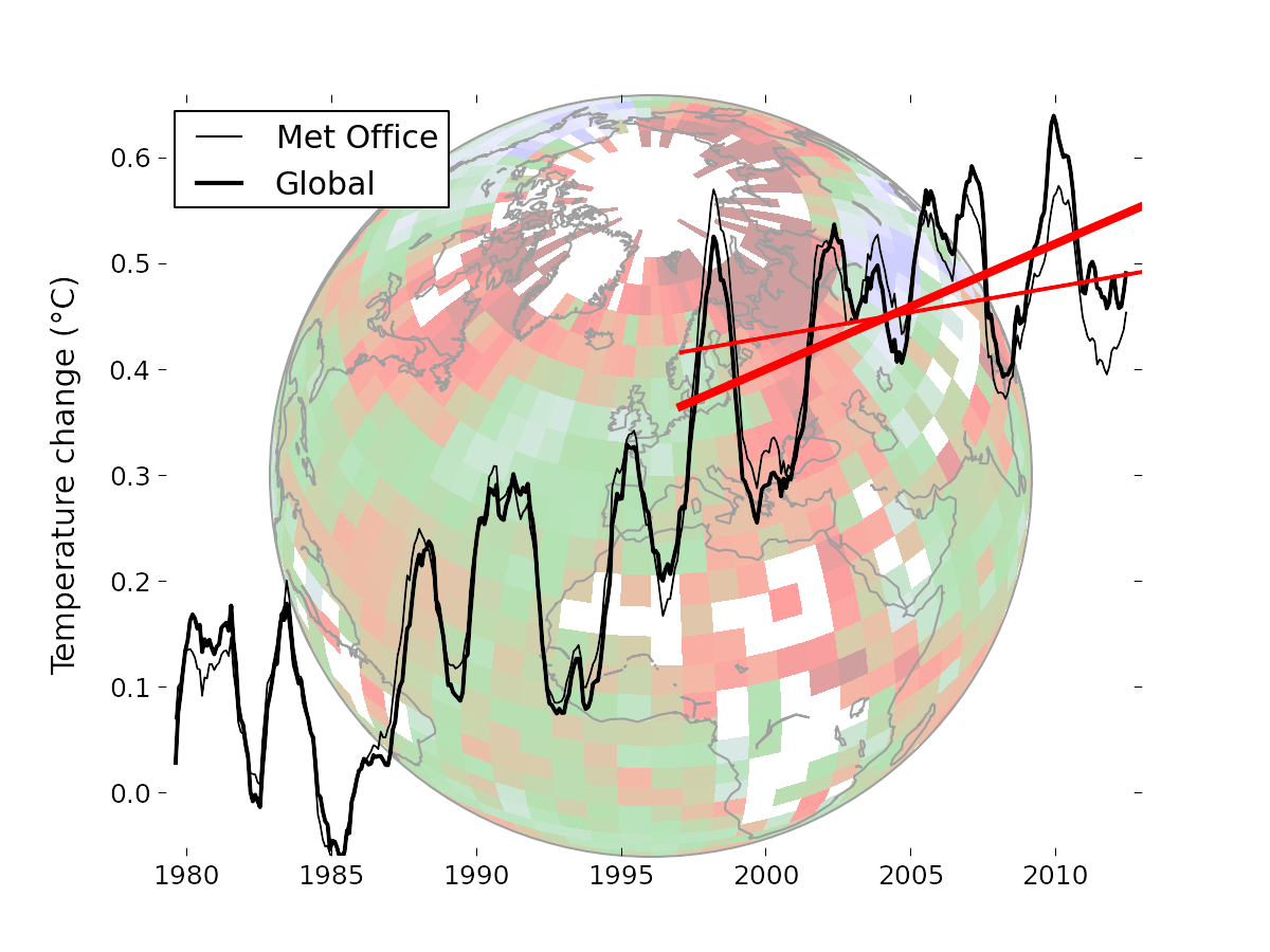
This image from the C&W site gives an idea of the coverage issue. There is a lot of missing data outside the polar regions, but it is not clear whether that biases the trend. But the polar regions are warming rapidly, and to in effect treat the missing cells as global average does create a bias.

I formed a latitude average for each month for a 5° band using the following weighting rules. Cells in that band with data have weight 1. Cells in adjacent bands have weight r, where r is typically 0.1-0.2. Cells in the band adjacent to that have weight r^2. Others are not used.

The point of this is that where there is good coverage, the average will be close to the band average. But if the central band has few data cells, the adjacent band cells, though downweighted, will be more significant by their numbers, avoiding the high variance that would come from relying on just the few cells in the central band. And if both those bands have few entries, then the third level comes into play. This is really only relevant to the N pole band, where the two bands above 80° are sparse.

I then simply infill missing data for each month with the latitude band average value, and compute trends for the resulting complete set.

I expect the result to vary little with r - this will be shown.

Results

The trend over the period 1997-2012, in °C/decade was:

HAD 4 cited C&W	0.046
HAD 4 with global average infill	0.0539
HAD 4 with lat av infill r=0.05	0.0854
HAD 4 with lat av infill r=0.1	0.0846
HAD 4 with lat av infill r=0.2	0.0821
GISS cited by C&W	0.080
C&W hybrid	0.1187

So this simple infill almost doubles the trend, but does not go as far as the C&W hybrid method. It is, however, close to GISS, which interpolates to avoid missing cells.

The graph by latitude band is



Here is a graph to show the small variations with different r (parameter for spreading estimate of latitude band average)

Conclusion

This shows that the trend is indeed biased by coverage. Using a latitude average estimate to replace missing values is at least as justifiable as the default global average. No special interpolation techniques are used, nor any alternative datasets. The change is substantial, though not as complete as C&W. However, the plot of trend by latitude bands is quite similar to the hybrid method.

October GISS Temp down by 0.13°C

GISS LOTI went from 0.74°C in September to 0.61°C in October. TempLS was fairly steady, satellites mixed.

GISS has been unusual lately among surface indices. You can see it here. While TempLS and NOAA have been fairly steady over the last five months, GISS went down, then up, and is back to where it started.



Here is the GISS map for Oct 2013:

And here, with the same scale and color scheme, is the earlier TempLS map:

Previous Months

September
August
July
June
May
April
March
February
January
December 2012
November
October
September
August
July
June
May
April
March
February
January
December 2011
November
October
September
August 2011

More data and plots

Cowtan and Way trends

A new paper by Kevin Cowtan and Robert Way in QJRoyMetSoc is getting a lot of discussion. See Real Climate here, SkS here and here, Lucia here and here, Cliamte Etc here.

The authors say:
"A new paper published in The Quarterly Journal of the Royal Meteorological Society fills in the gaps in the UK Met Office HadCRUT4 surface temperature data set, and finds that the global surface warming since 1997 has happened more than twice as fast as the HadCRUT4 estimate."

Some eyebrows have been raised at the size of the trend change from improving a relatively small area. I was surprised, too. So I did some calculations to see.

Update: The R code for calc and plotting is here. The data is provided by the authors here.

The need for the change

Met station coverage of the Earth is uneven. When grid averages are taken, and then combined for a hemisphere or global average, quite a lot of cells have no data. What to do?

The default is to leave them out of the average. But that is not a neutral decision. In arithmetical effect, they have been replaced by the average value of the cells with observations. And this may be a poor approximation. It should be improved with whatever information is available.

The particular issue with Hadcrut is data at the poles. In computing trends, missing cells are given the global average trend, but the poles are warming much faster. This is a big bias.

Cowtan and Way used UAH satellite data to get that improvement. I won't go into detail here about how they did it, but I'll just look at the dataset results. They looked in particulat at a period from 1997-2012 (16 years) which is commonly discussed as a pause. They showed trends including their hybrid method, which uses UAH-based infill:

Dataset	HADCRUT 4	UAH	C&W hybrid
Treend C/dec	0.046	0.094	0.119

Actually, I don't think they cited the UAH trend, but I calculated it from the data they used.

So the new trend isn't that much greater than UAH. But to see just how modifying polar trends made the difference, I'll show the latitude averages for the 5° ranges.

Latitude averages

In computing these for the HAD 4 data, I replaced data-free cells with the global average for that month. So they aren't a good guide (for HAD 4) to actual trends, but, as described above, they do correspond to what effectively goes into the global average, so you can see the effect of changes. Here's the plot:


(An earlier version of this plot had the sign of latitude wrong)

As you'll see, the Antarctic and Arctic trends for the hybrid are large, but not so very much larger than UAH. I am still a little surprised that this is so, but it's not unbelievable.

Appendix

Here are the numerical results as plotted:

Latitude	HAD 4	UAH	C&W hybrid
87.5	0.139	0.819	1.509
82.5	0.19	0.987	1.692
77.5	0.373	0.897	1.452
72.5	0.617	0.641	1.196
67.5	0.57	0.495	0.825
62.5	0.236	0.317	0.353
57.5	0.041	0.12	0.088
52.5	-0.083	0.05	-0.035
47.5	-0.056	0.013	-0.034
42.5	0.115	-0.028	0.102
37.5	0.061	0.026	0.066
32.5	0.067	0.131	0.074
27.5	0.085	0.104	0.086
22.5	0.051	0.068	0.091
17.5	0.074	0.009	0.09
12.5	0.085	-0.015	0.093
7.5	0.056	-0.008	0.059
2.5	-0.003	-0.027	-0.011
-2.5	-0.031	-0.017	-0.044
-7.5	-0.039	-0.037	-0.04
-12.5	-0.01	-0.039	-0.004
-17.5	-0.002	-0.028	0.01
-22.5	0.05	0.036	0.063
-27.5	0.088	0.062	0.093
-32.5	0.137	0.066	0.141
-37.5	0.082	0.053	0.094
-42.5	0.046	0.126	0.074
-47.5	-0.079	0.202	-0.048
-52.5	-0.114	0.215	-0.039
-57.5	-0.17	0.154	-0.041
-62.5	0.04	0.102	-0.009
-67.5	0.08	0.152	0.099
-72.5	0.079	0.569	0.566
-77.5	0.122	0.437	0.646
-82.5	0.086	0.299	0.685
-87.5	0.101	0.223	0.901
Global	0.054	0.094	0.119

TempLS global temp very small increase in October

The TempLS monthly global anomaly for October 2013 was 0.502°C, compared with 0.493° in September. TempLS has been very stable for the last five months. UAH showed a modest decrease.

Here is the spherical harmonics plot of the temperature distribution:
Update 18/Nov I see that by mistake I had link graphics for April in place of October. Fixed.




NW USA cold, SW Europe and central Asia warm..
And here is the map of stations reporting: