Reykjavik and GHCN adjustments.

There was a WUWT guest post recently by Paul Homewood on GHCN and GISS adjustments, and their effect on Iceland. It was somewhat along the lines of an earlier Eschenbach post on Darwin.

Then there were the usual thoughtful WUWT responses
When are the legal people going to be brought into this?
Someone should go to jail if this is tampering as it appears.
we’ve still a bunch of scumbags on this earth pretending that a dynamic history is OK
etc. So what happened

No, history was not rewritten. What the folks there don't seem to want to acknowledge is that GHCN circulates two files, described here. The file everyone there wants to focus on is the adjusted file (QCA). This, as explained, has been homogenized. This is a preparatory step for its use in compiling a global index. It tries to put all stations on the same basis, and also adjust them, if necessary, to be representative of the region. It is not an attempt to modify the historical record.

That record is contained on the other data file distributed - the unadjusted QCU file. This contains records as they were reported initially. It is generally free of any climatological adjustments. For the last 15 or so years, Met stations have submitted monthly CLIMAT forms. You can inspect these online. Data goes straight from these to the QCU file, and will not change unless the Met organisation submits an amended CLIMAT file. This is the history, and no-one is tampering with it.

The adjusted file does change, as the name suggests it may. Recently, it has been modified to use an improved pairwise comparison homogenization algorithm due to Menne and Williams. It is now (as of Dec 15 2011) used by GISS instead of their own homogenization algorithm, which makes the QCA file much more significant.

Update. I have a new post which looks at the GHCN adjustments more generally, with visualization.

The Iceland Met Office record

So Paul raised this with the Icelandic Met Office, with the following loaded questions:
a) Were the Iceland Met Office aware that these adjustments are being made?
No we were not aware of this.
b) Has the Met Office been advised of the reasons for them?
No, but we are asking for the reasons
c) Does the Met Office accept that their own temperature data is in error, and that the corrections applied by GHCN are both valid and of the correct value? If so, why?
The GHCN “corrections” are grossly in error in the case of Reykjavik but not quite as bad for the other stations. But we will have a better look. We do not accept these “corrections”.
d) Does the Met Office intend to modify their own temperature records in line with GHCN?
No.

And the Met sent their own version of the Reykjavik data. But what is missing from this dialog is that GHCN was never altering their QCU record, and is not suggesting that the Iceland records should be changed. I'll show the QCU data for the period most complained of, post 1939. Units are .01°C. Unfortunately, the Dec numbers got lost in formatting.

Year	Jan	Feb	Mar	Apr	May	Jun	Jul	Aug	Sep	Oct	Nov
1937	80	-160	-130	500	690	960	1160	1040	860	400	360
1938	10	180	200	470	600	920	1130	1060	940	490	170
1939	-150	130	360	500	870	1080	1300	1230	1180	740	150
1940	160	170	-20	300	760	970	1120	1010	710	630	130
1941	-30	-150	210	540	880	1150	1230	1150	1150	710	480
1942	160	190	270	360	770	970	1140	1130	790	260	410
1943	40	-90	150	290	500	990	1140	990	810	450	200
1944	-170	60	140	410	660	990	1300	1180	800	460	10
1945	-260	10	410	440	760	980	1190	1200	960	720	650
1946	240	-20	280	320	840	870	1060	1060	800	760	140
1947	320	-200	-280	170	830	990	1090	1100	770	560	30
1948	70	200	320	120	460	940	1060	1100	620	310	250
1949	-270	0	10	0	360	980	1050	1010	900	450	250
1950	280	-70	130	220	710	930	1240	1220	720	450	70
1951	-150	-90	-300	0	690	980	1060	1140	970	570	90
1952	-290	-30	100	340	620	830	1010	1010	760	570	260
1953	60	180	270	10	680	1020	1190	1150	970	420	200
1954	200	10	160	450	760	1020	1060	1100	610	370	270
1955	-200	-270	140	560	570	990	1050	1010	810	390	430
1956	-320	270	360	360	660	840	1070	990	930	470	500
1957	110	-150	40	500	700	990	1200	1130	710	470	300

Despite all the invocation of the Iceland data, there is no electronically readable form supplied. You can compare the link above, though, and you will see that the GHCN QCU data is almost identical. There are changes of a fraction of a degree - the Iceland Met do say that they have also made some adjustments.

Actually there are isolated differences. These seem to be sign differences, where GHCN has a negative sign. The sign may have disappeared in scanning the Iceland numbers.

The story of the Reykjavik adjustments was taken up by Ole Humlun, with again the same disdain for the record contained in the GHCN QCU file and the purpose of the homogenization adjustment. He refers to the Iceland data, and to Rimfrost, but does not mention the almost identical QCU.

The V3.1 adjustments

It is true that the adjustments have changed recently. V3.1 was released 4 November 2011. I have a QCA file from 14 July 2011, and this is, for Reykjavik, almost identical to the QCU file. I have a v2.mean file from Dec 2009, which is the V2 unadjusted file, and it is essentially identical to the current QCU file. In v2 style, it had duplicates. there were four for Reykjavik, but they had little overlap and where they did, were consistent. The unadjusted file has not changed, but the QCA file has.

I also have an adjusted v2 file from Dec 2009. The adjustments are substantial, but less than the current ones.

So here is the plot of the current QCU file vs the adjusted QCA file:



And here is the plot of differences



As you see, the adjustments are substantial. I have done a repeat of the GHCN analysis that we did for Darwin, with a histogram of the effect on trends. I will blog about this shortly. Current estimate is that this adjustment is in the top 10%.

December 2011 temp, small changes for NOAA, GISS

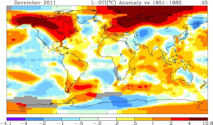
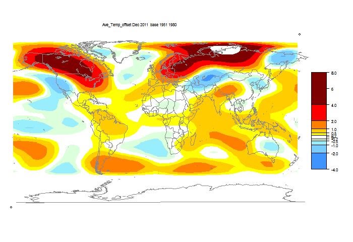
TempLS showed a very small rise in global mean anomaly in December, from 0.358 °C to 0.364 °C. Now NOAA and GISS are out. NOAA has a slightly larger rise, from  0.437°C to 0.457°C. And GISS has a small fall, from 0.48°C to 0.45°C. All these are relative to their respective base periods. Time series graphs are shown here

As usual, I compare the previously posted TempLS distribution to the GISS plot. Here is GISS:







And here is the TempLS spherical harmoics plot:

Previous Months

November

October

September

August



More data and plots

Lapse rates and entropy.

The dry adiabatic lapse rate (DALR) is in the news again. Willis Eschenbach has led a discussion primarily directed at a theoretical musing on whether gas under gravity but without heat input would have a lapse rate or be isothermal.

I've explained my views on the role of the DALR here and here, and in comments on several other blogs. Just a brief recap of theory; the DALR is the vertical temperature gradient given by:
dT/dz = -g/c_p = -9.8 °C/km for air,
where z is altitude, g gravity acceleration, and c_p is the (constant pressure) specific heat of air. Any gas cools when it expands adiabatically (ie without exchanging heat with the environment). The rate at which dry air cools as it rises (and the pressure falls) is also the DALR.

The air generally does have a lapse rate which is not quite as large as the DALR. This observed rate is called the environmental lapse rate. The difference is often attributed to the effect of water condensation, and there is reference to a moist adiabatic lapse rate. I think that is only part of the story, as I'll show.

But my view of the role of the DALR, and the answer to Willis' query, is fairly simple. Air motions create a heat pump which move temperatures toward the DALR. If you could prevent all motion, conduction would move the temperature gradient to isothermal. But you can't; in practice the air needs heating to keep it from liquefying, and that will always create motion.

In this post, I'll review the heat pump notions, and add an entropy viewpoint which will quantify some of the issues.

The heat pump of moving air.

I've talked about that in the previous posts referenced above. For here, I'll just repeat part of a comment I made at WUWT

When the lapse rate is below the dry adiabat (toward isothermal) it is referred to as convectively stable. Above the adiabat, it is unstable. At the adiabat, it is neutrally stable.

At the adiabat, rising air cools by expansion, at exactly the rate at which the nearby air is becoming cooler (by lapse rate). And falling air warms. There is no buoyancy issue created. Moving air retains the same density as the environment. And no heat is transferred.

But in the stable regime, falling air warms faster than the change in ambient. It becomes less dense, so there is a force opposing its rise. That is why the air is stable. This motion both takes kinetic energy from the air and moves heat downwards (contra your statement). It is a heat pump which works to maintain the lapse rate.

Rising air does the same. It cools faster, and so rises against a buoyancy force. It takes KE from the air and moves “coolness upwards”, ie heat down. It pumps heat just as falling air does.

That is why air in motion tends to the adiabat lapse rate. A heat pump requires energy. Where from?

The atmosphere is famously a heat engine, driven by temperature differences, most notably from equator to pole, but also innumerable local differences, eg land/sea. This provides the kinetic energy that maintains the lapse rate, and it is hard to imagine any planetary atmosphere where the energy would not be available.

The effectiveness of the heat pump tapers as the adiabat lapse rate is approached. Beyond, in the unstable region, everything is reversed. The pump becomes an engine, with heat moving upward creating KE. This of course quickly diminishes the temperature gradient.

Entropy

As said above, a heat pump is needed to maintain a lapse rate. The reason is that there is the irreversible process of conduction down the temperature gradient:

Q = -k ∇T

where k is the thermal conductivity (W/m/°K), and Q is the flux. This is a general Fourier law, and k need not be simply molecular conductivity. For present purposes it is augmented by turbulent transfer and also by radiative transfer if there are GHGs.

I'm using "irreversible" in the thermo sense; heat flow down the gradient can be (and is) reversed by a heat pump. But that takes energy.

Since the Fourier law flow is irreversible, it creates entropy:

dE_A/dx = Q d(1/T)/dx, where E_A is a time rate of increase of entropy per unit area, or more conveniently (see Eq 3):
E_V = (k/T²) ∇T • ∇T, where E_V is the rate of entropy increase per unit volume.

As you see, E_V depends only on k and the temperature and its gradient. It happens inexorably, with or without gravity. You can only reach a steady state if you either

• have gradient zero
• have k=0 or
• use energy to counter the entropy increase

The adiabatic heat pump does counter the entropy increase. But of course, globally entropy grows. The energy for the heat pump comes from air motion created by the global atmospheric heat engine, which necessarily creates at least as much entropy as the heat pump negates. And that entropy is ultimately exported from the Earth.

Environmental lapse rate

The observed lapse rate is usually less than the DALR, and this is often attributed to moisture. There isn't actually a "moist adiabatic lapse rate" that you can cite a value for. But one way of seeing how moisture could matter is if you think of the role of specific heat. This is just the amount of heat needed to change the temperature, and during condensation, you can say that the specific heat experiences a spike - effectively a delta function with area LH. When the SH rises, g/c_p diminishes. But the moist adiabat does require that condensation is actually happening, and of course in the air that happens only in some places at some times.

But another reason for the lapse rate falling short of the DALR is simply that the heat pump is inadequate. It's effectiveness tapers to zero as the lapse rate approaches the DALR. But in fact the rate of entropy creation that it has to counter is quite high when GHG are present, because of radiative transfer (Rosseland conduction). And as above, to the extent that it is inadequate, the temp gradient tends toward isothermal.

December TempLS surface temp - little change

A very small rise in global mean anomaly this month, from 0.358 °C to 0.364 °C.

Below is the spherical harmonic regional distribution. Some very high anomalies in Siberia and NW Canada.

Previous Months

November
October
September
August

More data and plots

Cherrypicker's guide to station trends

Cherrypicker's guide to station trends

A while ago I posted a cherrypicker's guide to global surface temperature trends. This was partly in response to an outburst of the popular activity of selecting short periods where the trend could be seen as small or even negative. The idea was to embed this in a set of displayed results where you could get a broader picture of where such trends might be found, and how significant the regions were

Another popular activity is selecting stations which fail to show recent warming. So I've presented here a different kind of plot which shows all the GHCN stations on a world map, with shading to indicate the trend over the last 30, 45 or 60 years (you can choose). It derives from the plot I posted for November temperatures. It takes advantage of HTML 5 linear color shading, and uses a triangular mesh. Each station has a color corresponding to its trend for the chosen period; although the colors can vary locally, the station neighborhood itself should have the correct color. Note that there is no spatial averaging (except for the shading); the individual station trends determine the coloring.

One result that I found interesting is that while there are patchwork regions, eg USA, there are also large regions with fairly uniform trends, particularly the ocean.

So here's the plot. It is interactive - you can rearrange it, magnify, show the stations, click to see station detail and numbers etc. Use Ctrl+. Ctrl- to get it the right size for your screen. The mechanics are explained below.

your browser does not support the canvas tag

Click on this map to orient the world plot. Show Stations Show Mesh Magnification 2× 4× Trend period 1951-2010 1966-2010 1981-2010 Station

How it works

More details here. The flat map at top right is your navigator. If you click a point in that, the sphere will rotate so that point appears in the centre. The buttons below allow modification. Set what you want, and press refresh. You can show stations, and the mesh, and magnify 2×, 4×, or 8× (by setting both). You can click again to unset (and press refresh). Then you can click in the sphere. At the bottom on the right, the nearest station name and anomaly will appear. You may want to have stations displayed here. The selection menu chooses the period; if you change the period, the plot changes without need for refresh.

How the trends are calculated.

Calculating station trends is not trivial, because of missing values and seasonal variation. Obviously missing winter values at one end will bias the trend. A reasonable fix is to subtract the mean for each month and work with anomalies. But the means don't correspond exactly to the same period. I used a weighted least squares method similar to that used in TempLS. The weighting simply has unit value for months with readings, zero without. The model is x_my  ~  L_m  +  Tr  J_my where x are the station readings, L the monthly offsets, Tr the trend, and J a linear progression of months, in century units. The suffixes m for month, y for year. This is fitted by least squares. The resulting formula is similar to OLS. If we now say that J has zero values for missing x, and I is a similar vector which is 1 mostly, but zero where x is missing, then the OLS trend formula would be

Tr = f(x) / f(J)  where   f(x) = S(Jx) - S(J) S(x) / S(I)

where S represents summation over all month/year. Denoting S_y as the process of summing over individual months, and S_m summing the resulting 12 sums, the formula from the above fit is:

Tr = f(x) / f(J); f(x) = S(Jx) - S_m( S_y(J) S_y(x) / S_y(I))

Data issues.

The data sets associated with these plots are getting larger, so attention to download time is needed. I'd like to be able to use gzip compression, but neither of the data stores I currently use support that. I have to send the data as text - basically Javascript assigns - so I use various tricks to get the text size down. I multiply by 100, say, to get rid of decimal points. I usually convert data to differences to make the numbers smaller. In fact, the biggest data item here is the world map. But potentially another big one is the triangle mesh, and there I had to make some compromises. I don't want to send a different mesh for each trend period, but if I send a mesh with all points, then in any one period, some stations will be missing. I dealt with this by using an interpolated value for coloring purposes. That's OK - the shading otherwise uses linear interpolation. But this isn't quite linear, and could look odd at times, though I haven't noticed anything. The missing (interpolated) stations don't appear when stations are shown, and are not reported when station values are produced by clicking. Anyway, the datafile size is now about 360 Kb, which is manageable. I'm looking out for better ways because I have ambitions that involve transmitting the whole TempLS dataset.

Notes

You may see a few ocean stations appearing on land. The reason is that I artificially create ststions at the centre of each 4x4 deg cell. If there is enough sea in the cell for HADSST to report a SST value, that will be assigned to that central point, even if it is on land.


Note that the color scheme suggests cooling, but most of the blue range is actually positive (though smaller) trend.


Stations are included in the trend analysis if they have at least 80% of months reporting within the range.