<h2>Moving to FEM variant of TempLS global temperature average.</h2>

TempLS is my least squares based global temperature anomaly calculating program which I use to post each month's anomaly as station data from GHCNV4 unadjusted and ERSST become available. I have four different methods for the basic step of integrating the temperatures based on the irregular sampling points. Of these, the FEM method is most recent, and is described here.

There isn't a pressing need for a new method. The existing methods agree with each other to a few hundredths of a degree, and I think are capable of equal accuracy. The mesh method was the first of the advanced methods I used, and has remained the workhorse. It is the slowest, but speed is not really an issue. It takes about an hour to process all data since 1900. But all methods are based on representing the integral as the weighted sum of temperatures, and the weights depend only on the location of stations. The station set in months before the last few years rarely changes, and so the weights can be stored. It is calculation of the weights that consumes most time. With stored weights, all methods take only a minute or two to process the complete data set.

However, the FEM method is tidier and easier to maintain. An issue with the mesh method is that it does not make a very good map of temperatures, and so I import LOESS data for that. The FEM method can easily be tweaked to produce very good maps. And it is a lot faster.

Overview of methods

As described in the TempLS Guide and other articles linked there, TempLS works by fitting a linear model to the measured temperature
T_smy=L_sm+G_my
Subscript s for station, m for month, y for year. The L's are called offsets, but they play the role of normals, being independent of year. G, depending on time but not s, is the global temperature anomaly. L and G are determined by minimising a weighted sum of squares, weighted to represent a spatial integral. This fitting is common to all methods; the differences are just in the determination of the weights.

Grid method and infilling

The method everyone starts with is just to form a grid, and assign to each cell the average temperature of the measurements within. The weights are the cell areas. The fitted function is thus piecewise constant, and discontinuous, which is not desirable. But the main weakness is that some cells may have no data. The primitive thing is just to omit them from the average (Hadcrut did that until the recent V5). But the obligation is to give the best estimate of each cell, and omitting just says that those cells behave like the average of the others, which may be far from the truth.

This can be made into a good method with infilling. I use Laplace equation solution, which in practice says that each missing cell value is the average of its neighbors. That requires iterative solution. But then it is accurate and fast. I use a grid which is derived from a gridded cube projected on the sphere (cubed sphere).

Irregular mesh

My next method was to join up the stations reporting in each month in a triangular mesh (convex hull), and interpolate linearly within each triangle. That leads to a continuous approximating function, which is good. The meshing is time consuming (a full run takes over an hour on my PC), but does not have to be repeated for historic months for which there is no change in stations. The weights work out to be the areas of triangles of which each station is part.

This method is excellent for averaging, but gives poorly resolved maps of temperature. For that I had been using results from the next method, LOESS.

LOESS method.

This uses a regular icosahedral mesh to get evenly spaced nodes. The node values are then inferred from nearby station values by local weighted regression (first order, LOESS). Finally the node values are integrated on the regular mesh.

The method is fairly fast, and there is a lot of flexibility in deciding how far to search for neighboring points. An oddity of the method is that it can yield negative weights, which can be a problem for the model fitting (but usually isn't).

The FEM method

Details here. It isn't strictly FEM, but uses the basis functions of FEM on a regular icosahedral mesh. I generally use linear functions, but higher order can be more efficient. For linear each basis function is a pyramid centered at a node and going from one to zero on the far side of each triangle. The parameters are the nodal values, which are also the multipliers of the basis functions.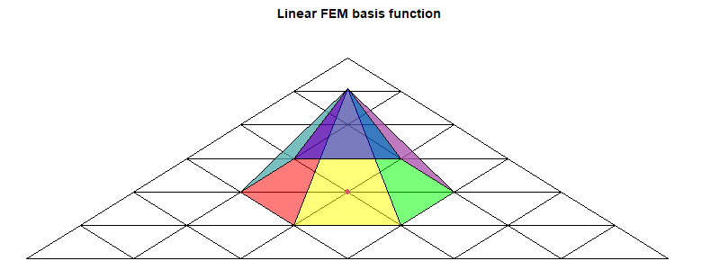



The objective is to find those parameters b that minimise ∫(T(x)-b.B(x))²dx over the sphere, where B is the vector of basis functions. T(x) of course is known only at sample points, so the discrete sum to minimise is
w_(i)(T(x_i)-b_jB_j(x_i))²
I am using here a summation convention, where indices that are repeated are summed over their range. The weights w_(i) are those to approximate the integral; the suffix is bracketed so that it is not counted in the pairing (summation). The weights here are less critical; I use those from the primitive grid method.

The minimum is where the derivative wrt b is zero, giving the familiar regression expression:
w_(i)(T(x_i)-b_jB_j(x_i))B_j(x_i)=0
or
B_kiw_(i)B_jib_j=B_kiw_(i)T(x_i) where B_ki is short for B_k(x_i)
B_kiw_(i)B_ji may be shortened to BwB_kj. It is a symmetric matrix, and positive definite if the w_(i) are positive. Solving for b:
b_k=(BwB^-1)_kjB_jiw_(i)T(x_i)
BwB has a row and column for each basis function, so it can be a manageable matrix. But I tend to use the preconditioned conjugate method, without explicitly forming BwB. It usually converges well, and so is faster. I'll say more about this in the appendix

There are two ways this equation for b is used:

• The expression for the global integral of T is a_kb_k, where the a's are the integrals of each basis function. So the integral can be written as a scalar product W_iT(x_i). The weights W are just what is needed for the final stage of TempLS iteration, and so are given by
  a_k(BwB^-1)_kjB_jiw_(i)
  This is evaluated from left to right.
• For mapping the anomaly, evaluation goes from right to left, starting with known anomalies in place of T. The result is the basis function multipliers b, which can then be used to interpolate values, and so colors, to pixel points.

In either case, the key step is the solving with BwB. The rest is just scalar products.

Summary

I am planning to use the FEM method for global temperature calculation because with the same operators I can also do interpolation for fine-grained graphics. The method is accurate, but so are others; it is also fast. Higher order FEM would be more efficient, but first order is adequate.

Appendix 1 - sparse multiplication

I'll describe here two of the key tools that I have developed in R, which are fast and simplify the coding. The first is a function spmul, which multiplies a sparse matrix A by a vector b.

The matrix A is represented by a nx3 matrix C, with a row for each non-zero element of A. The row contains first the row number of the element, then the column number, and finally the value, The length of b must match the number of columns of A.

The rows of C can be in any order. spmul starts by reordering so that C[,1] is in ascending order, so each bunch of equal values corresponds to a row of A. To get the row sums of A, the operator cumsum is applied to C[,3]. Then the values at the ends of each row bunch are extracted and differenced (diff). That gives the vector of row sums.

The same steps are used to multiply A by b, except the values are first multiplied by b[C[,2]].

There is a twist that A may have empty rows, with no entry in C. That can mostly be handled by using the values in reordered C[,1] to place results in a vector initially filled with zeroes. But if final rows of A are missing, this won't work, because C does not tell how many rows there should be. This can be given as an optional extra argument to spmul.

Preconditioned conjugate gradient method

This is described in wiki here. I follow that, except that instead of argument A being a matrix, it is a function operating on a vector (the function must of course be self-adjoint and positive definite). In that way the sequence B_kiw_(i)B_ji can be given as a function to be evaluated within the algorithm.

My preconditioning is actually minimal - diagonal at best, although even no preconditioning works quite well.