<h2>Airborne fraction CO2 and the Bern model</h2>

We've been discussing IPCC projections and RCPs in relation to the airborne fraction (AF) of CO2. The AF is the fraction of CO2 emitted that remains in the air, relative to the amount emitted. In an earlier post I showed that if you plotted cumulative emissions against total CO2, it was very linear, implying a close to constant AF. You get different constants depending on whether you look at just FF emissions, or total, including land use.

At first constant AF might seem to be a consequence of Henry's Law. But that gives a fixed phase partitioning at equilibrium, which we don't have (not to mention acid/base chemistry). It might seem surprising that the time varying sink uptake could give that result.

So I tried with the dynamics of the Bern model. This is what the IPCC would probably use if they were to express an opinion on the future of AF (which they don't). The Bern model yields an impulse response function for a pulse of CO2 injected into the atmosphere. In this version, it makes that out of the sum of decaying exponentials of periods ∞, 171, 18 and2.57 years. If you filter total emissions with this function (reversed), that gives the modelled growth of the amount of CO2 in the air at any time. A caveat; fitting observed AF was no doubt one of the considerations in designing the Bern model.

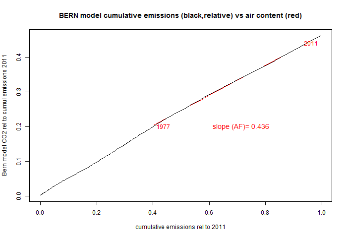
So I did that. I'll show the results below. Plotting accumulated CO2 against cumulative emissions, the result is still remarkably linear. And the slope, at 0.436, is remarkably close to what I found with observed CO2 (0.439). OK the caveat applies, but the constancy is the real result.

The above link gives the time constants, formula, includung the corresponding weights: (0.152, 0.253, 0.279 and 0.316). I should mention that the weighted sum of exponentials does not offer much uniqueness; especially with all positive coefficients, various decay constants could give similar results. There is no orthogonality. So it's unwise to try to over-interpret their meanings; what matters is that they provide a valid approximation.

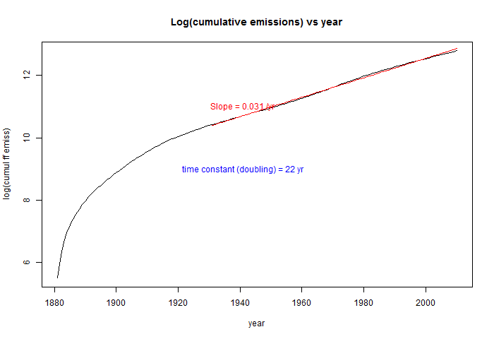
Note too that the impulse response does not have an integral (to ∞) since it does not tend to zero. So to get results, we rely on the emissions starting from near zero some finite time back. The emissions are total to 2011, including land use, as described here. The growth is in fact near exponential, as its linearity in the following log plot shows:



So here now is the plot of accumulation vs emissions. I've normalised by dividing by the total emissions to date. I show a linear regression from 1977 to 2011, which is the highly linear recent section:



Mathematically, the reason for the linearity is associated with the exponential increase. You can do the integration directly to get a result as a rational function of the time constant; this varies quite slowly.